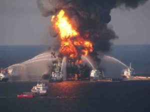
Home Blog Page 69

Rewriting the textbook on fossil fuels

Abiotic sources of methane have been found in more than 20 countries and in several deep ocean regions so far. Credit: Deep Carbon Observatory

Experts say scientific understanding of deep hydrocarbons has been transformed, with new insights gained into the sources of energy that could have catalyzed and nurtured Earth’s earliest forms of life.

During the past hundred years scientists worked out in detail how hydrocarbons—fossil fuels” drawn from reservoirs in Earth’s crust to heat and power homes, vehicles, and industry—have a biotic origin, derived from the buried plants, animals, and algae of eons past.

But for some hydrocarbons, especially methane—the colorless, odorless main ingredient in natural gas—nature has many recipes, some of which are “abiotic—derived not from the decay of prehistoric life, but created inorganically by geological and chemical processes deep within the Earth.

Abiotic hydrocarbons have been a major focus of the Deep Energy community of the Deep Carbon Observatory program—a 10-year exploration of Earth’s innermost secrets, concluding in October.

DCO experts believe an abiotic origin of methane explains most of the unusual occurrences of the gas, including the flames of Chimaera in southwest Turkey.

Chimaera does not sit atop conventional deposits of oil and gas produced from the decayed organic residue of earlier epochs. And yet, dozens of small fires have burned at this mountaintop site for millennia.

Ancient explanations for the flames included the breath of a monster—part lion, part goat, part snake. The less colorful scientific reason: highly flammable abiotic methane and hydrogen rising to Earth’s surface from deep below.

Chimaera is among the most photogenic and famed of now hundreds of sites where abiotic sources of methane have been found in more than 20 countries and in several deep ocean regions so far.

DCO collaborator Giuseppe Etiope of the Istituto Nazionale di Geofisica e Vulcanologia in Rome has documented the Chimaera site and several other environments at which unusual occurrences of methane have been found, including:

  • Ancient Precambrian shields—rock at the core of the continents formed as much as 3 billion years ago
  • On the ocean floor (e.g., high-temperature vents on and near mid-ocean ridges and belching mud volcanoes)
  • On continents (seeps and hyper-alkaline springs and aquifers).

While diverse rock types are present in all these environments, he notes, many discoveries have focused on places with specific, suitable types of “ultramafic” rocks such as peridotite (a coarse-grained igneous rock) included in massifs and ophiolites (ensembles of rocks formed from the submarine eruption of oceanic crustal and upper mantle material).

Earth’s abiotic methane is now thought mainly to derive chemically from the hydrogen created by the hydration of ultramafic rocks undergoing “serpentinization”—a reaction that occurs when water meets the mineral olivine.

Hydrogen also nourishes biological sources of methane. DCO researchers have documented a vast microbial ecosystem—a deep biosphere fed by hydrogen. Many of the deep microbes, called methanogens, metabolize hydrogen to produce methane.

The deep biosphere has therefore posed a chicken and egg scenario: which came first, abiotic methane or microbes? If abiotic methane came first, as seems obvious, did it give rise to Earth’s first microbes? And if microbes came first, how and why did they inhabit places almost devoid of sustenance?

A decadal goal: sort out the origins of methane on Earth

When the Deep Carbon Observatory project began in 2009, DCO’s Deep Energy community—now made up of more than 230 researchers from 35 nations, set the decadal goal of sorting out the origins of methane on Earth.

Some hypothesized that unusual methane reservoirs—i.e., those that could not be biotic in origin—must form through chemical reactions occurring in the surrounding rocks.

Others suggested that microbes contributed to methane production in some reservoirs, metabolizing hydrogen to create methane in an entirely different process.

Others hypothesized that methane might originate deeper in Earth, in the upper mantle, and diffuse up toward the surface. (At Moscow’s Gubkin University, researcher Vladimir Kutcherov is leading experiments to test the production of methane in lab-simulated high-pressure conditions of Earth’s upper mantle).

Early in its mandate the DCO made the decision to invest in new analytical instrumentation to overcome some of the limitations to deciphering the origin of methane.

With strategic investment in instrumentation and numerous field samples, DCO partners set out to pioneer new investigative tools to distinguish Earth’s biotic from abiotic methane.

In 2014, three new instruments came online with the potential to change the face of deep carbon science, and they have not disappointed, says Edward Young, of the University of California, Los Angeles (UCLA), co-leader of DCO’s Deep Energy Community with Isabelle Daniel of the Claude Bernard University Lyon 1 in Lyon, France.

Using complementary techniques of mass spectrometry and absorption spectroscopy, scientists at UCLA, the California Institute of Technology (Caltech), Pasadena CA, and the Massachusetts Institute of Technology (MIT), Cambridge MA, are analyzing natural methane samples to better understand how abiotic methane may be produced.

“A molecule of methane (CH4) appears remarkably simple, made up of only five atoms,” says Dr. Young. “Rare isotopes of both hydrogen and carbon are occasionally incorporated into methane molecules, however, and the frequency of these ‘heavy’ isotopes reveals the secret of how they formed and at what temperatures.”

Of particular diagnostic value are methane molecules that contain more than one “heavy” isotope (“clumped isotopes”). These molecules are extremely rare and can only be distinguished by instruments with extremely high mass resolution, sensitivity, and power.

DCO collaborators used samples of gases collected from Chimaera, the deep mines of Canada, the Oman ophiolite, hydrothermal vents on the ocean floor, and additional sites, and were surprised by what they found.

Though interpreting the data is challenging, it appears microbes may be doing more than originally thought.

How much abiotic methane?

“We see curious biological fingerprints in samples that otherwise appear to have an abiotic signature,” says Dr. Daniel. “It seems microbes know how to use these abiotic compounds as fuel.”

“We have clear and growing evidence of abiotic methane on Earth. What is not clear is how much there is. These investigations have found incredible complexity in the way methane is produced, and these complexities connect inorganic and organic chemistry on Earth in fascinating ways.”

Adds Dr. Young: “We went into this project thinking we knew how abiotic methane formed. What we’re learning is that it is much more complicated, and the biggest key is hydrogen. With greater understanding of how rocks make the hydrogen from which methane derives, and how fast this reaction happens, we’ll be a lot closer to knowing how much methane there is on Earth.”

Jesse Ausubel of The Rockefeller University in New York notes that the popular definition of “fossil fuel” doesn’t cover abiotic methane.

“Thousands of samples from many settings tested with super-sensitive instruments are producing a global picture of the abundances and fluxes of deep energy. Much of the very deep hydrocarbons is not conventional fossil fuel, as popularly defined.”

The behaviors of biotic and abiotic methane, it should be noted, in terms of energy output and emissions when burned, are indistinguishable.

Key findings to date:

  • Thanks to new instruments, scientists have identified new isotope signatures in methane to help determine its provenance—an impossibility 10 years ago
  • The serpentinization reaction is better understood and is one of several ways Earth’s rocks produce molecular hydrogen—a key source of geologic energy for the deep biosphere
  • That hydrogen reacts with carbon dioxide to produce methane was long known. How this happens in Earth’s crust, however, is highly complex, and many other organic molecules are created as byproducts in the process. These molecules can be used by microbes as a food source. They also represent intriguing clues as to the origins of life on Earth, as these organic molecules may be precursors for the building blocks of life (e.g., amino acids)
  • With similar conditions and reactions likely on other planets and moons (e.g., the subsurface of Mars or on the ocean floor of Enceladus), it strengthens the potential identification of where life may exist elsewhere in the universe
  • Studies of serpentinizing systems have found other abiotic hydrocarbons in addition to methane.

Future implications:

These investigations into how abiotic methane forms on Earth are not the end of the story, but rather the beginning.

The last 10 years have seen transformational changes in our understanding of the origins of methane on Earth and its pivotal role in sustaining the deep biosphere, providing a glimpse into the geological processes that could have set the stage for life.

With these new discoveries, we are poised to answer numerous big questions, such as:

  • How much abiotic methane is being produced in Earth?
  • How much methane do the microbes of Earth’s deep biosphere produce?
  • How much do the microbes consume?
  • What are movements and fates of abiotic methane?and
  • Where is abiotic methane stored and for how long?

The success of the project’s research has not only changed perceptions of energy generation in deep Earth, but also about how life may have found a foothold on our planet.

And if abiotic energy does occur on Earth, how likely is it that similar reactions and life have occurred elsewhere in the cosmos?

This Deep Energy research released today is a result of the Deep Carbon Observatory program, which will issue its final report in October 2019 after a decade of work by a global community of more than 1000 scientists to better understand the quantities, movements, forms, and origins of carbon inside Earth.

Reference:

  1. The contribution of the Precambrian continental lithosphere to global H2 production
    Sherwood Lollar, B., Onstott, T.C., Lacrampe-Couloume, G., and Ballentine, C.J. (2014). Nature 516 (7531): 379-382.
  2. Formation temperatures of thermogenic and biogenic methane
    Stolper DA, Lawson M, Davis CL, Ferreira AA, Santos Neto EV, Ellis GS, Lewan MD, Martini AM, Tang Y, Schoell M, Sessions AL, Eiler JM (2014). Science 344:1500-1503
  3. Measurement of a doubly-substituted methane isotopologue, 13CH3D, by tunable infrared laser direct absorption spectroscopy
    Ono S, Wang DT, Gruen DS, Sherwood Lollar B, Zahniser M, McManus BJ, Nelson DD (2014), Analytical Chemistry, 86:6487-6494
  4. Panorama, a new gas source, electron impact, double-focusing, multi-collector mass spectrometer for the measurement of isotopologues in geochemistry
    Young ED, Freedman P, Rumble D, Schauble E (2014), 7th International Symposium on Isotopomers (ISI2014), Tokyo, Japan
  5. The relative abundances of resolved 12CH2D2 and 13CH3D and mechanisms controlling isotopic bond ordering in abiotic and biotic methane gases
    Young E.D., Kohl I.E., Sherwood Lollar B., Etiope G., Rumble III D., Li S., Haghnegahdar
  6. M.A., Schauble E.A., McCain K.A., Foustoukos D.I., Sutclife C., Warr O., Ballentine C.J., Onstott T.C., Hosgormez H., Neubeck A., Marques J.M., Pérez-Rodríguez I., Rowe A.R., LaRowe D.E., Magnabosco C., Yeung L.Y., Ash J.L., Bryndzia L.T. (2017). Geoch. Cosmochim. Acta, 203, 235-264.
  7. Natural gas seepage, the Earth’s Hydrocarbon Degassing
    G. Etiope. (2015), Springer, Switzerland
  8. Widespread abiotic methane in chromitites
    Etiope G., Ifandi E., Nazzari M., Procesi M., Tsikouras B., Ventura G., Steele A., Tardini R., Szatmari P. (2018). Scientific Reports, 8, 8728, DOI: 10.1038/s41598-018-27082-0.
  9. Massive production of abiotic methane during subduction evidenced in metamorphosed ophicarbonates from the Italian Alps
    Vitale Brovarone A, Martinez I, Elmaleh A, Compagnoni R, Chaduteau C, Ferraris C, Esteve I (2017). Nature Communications 8:14134 DOI: 10.1038/ncomms14134
    Abiotic formation of condensed carbonaceous matter in the hydrating oceanic crust
  10. Sforna MC, Brunelli D, Pisapia C, Pasini V, Malferrari D, Ménez B. (2018). Nature Communications DOI: 10.1038/s41467-018-07385-6
  11. Abiotic synthesis of amino acids in the recesses of the oceanic lithosphere
    Ménez B, Pisapia C, Andreani M, Jamme F, Vanbellingen QP, Brunelle A, Richard L, Dumas P, Réfrégiers M. (2018). Nature DOI: 10.1038/s41586-018-0684-z
    Abiotic methane on Earth
    Etiope G, Sherwood Lollar B (2013). Reviews of Geophysics DOI: 10.1002/rog.20011
  12. Formation of abiotic hydrocarbon from reduction of carbonate in subduction zones: Constraints from petrological observation and experimental simulation
    Tao R, Zhang L, Tian M, Zhu J, Liu X, Liu J, Höfer HE, Stagno V, Fei Y (2018) Geochimica et Cosmochimica Acta 239:390 DOI: 10.1016/j.gca.2018.08.008
  13. Immiscible hydrocarbon fluids in the deep carbon cycle
    Huang, F., Daniel I., Cardon H., Montagnac G., Sverjensky D. (2017) Nature Communications 8:15798 DOI: 10.1038/ncomms1579
  14. Methane-derived hydrocarbons produced under upper-mantle conditions
    A. Kolesnikov, V.G. Kutcherov, A.F. Goncharov (2009) Nature Geoscience 2: 566-570
  15. Synthesis of Complex Hydrocarbon Systems at Temperatures and Pressures Corresponding to the Earth’s Upper Mantle Conditions
    V.G. Kutcherov, A. Kolesnikov, T.I. Dyugheva, L.F. Kulikova, N.N. Nikolaev, O.A. Sazanova, V.V. Braghkin (2010). Doklady Physical Chemistry 433:132-135

Note: The above post is reprinted from materials provided by Deep Carbon Observatory .

Uncovering Polynya : Research unravels 43-year-old mystery in deep Antarctica

Polynya
Maud Rise Polynya of September 2017 (the ice-free area near the yellow star) seen from space. Credit: SCAR ATLAS

A study led by NYU Abu Dhabi (NYUAD) Research Scientist Diana Francis has unraveled the four decade long mystery surrounding the occurrence of a mid-sea Polynya – a body of unfrozen ocean that appeared within a thick body of ice during Antarctica’s winter almost two years ago.

The Maud-Rise Polynya was spotted in mid September 2017 in the center of an ice pack in Antarctica’s Lazarev Sea, causing researchers to question how this phenomenon occurred during Antarctica’s coldest, winter months when ice is at its thickest. Due to its difficult access location, NYUAD scientists used a combination of satellite observations and reanalysis data to discover that cyclones (as intense as category 11 in the Beaufort Scale) and the strong winds that they carry over the ice pack cause ice to shift in opposite directions, which leads to the opening of the Polynya.

At the time of the discovery, the Maud-Rise Polynya was approximately 9,500 square kilometers large (equivalent to the landmass of the state of Connecticut), and grew by over 740 percent to 800,000 square kilometers within a month. Eventually, the Polynya merged with the open ocean once the ice started to retreat at the beginning of the austral summer months. Prior to 2017, this phenomenon has only been known to have occurred in the 1970s when satellite observations started to become more commonly used, and has baffled scientists ever since.

“Once opened, the Polynya works like a window through the sea-ice, transferring huge amounts of energy during winter between the ocean and the atmosphere.” said Francis. “Because of their large size, mid-sea Polynyas are capable of impacting the climate regionally and globally as they modify the oceanic circulation. It is important for us to identify the triggers for their occurrence to improve their representation in the models and their effects on climate.

“Given the link between Polynya and cyclones we demonstrated in this study, it is speculated that Polynya events may become more frequent under a warmer climate because these areas will be more exposed to more intense cyclones. Previous studies have shown that under warmer climate, polar cyclone activity will intensify and extratropical cyclones track will move toward Antarctica which could decrease the sea-ice extent and make Polynya areas, closer to the cyclones formation zone,” she added.

Reference:
Journal of Geophysical Research: Atmospheres, DOI: 10.1029/2019JD030618

Note: The above post is reprinted from materials provided by New York University.

Minerals in mountain rivers tell the story of landslide activity upstream

Himalaya
Mountains Annapurna South and Hiunchuli from near Ghandruk in the Himalaya of central Nepal. Credit: David Whipp

Researchers from the University of Helsinki and the University of Tübingen have come up with a new way of analysing sand in mountain rivers to determine the activity of landslides upstream, which has important implications for understanding natural hazards in mountainous regions.

Landslides occur in hilly and mountainous landscapes, often triggered by extreme rainfall events or ground shaking resulting from earthquakes. For example, a magnitude 7.8 earthquake in Nepal in April 2015 and its aftershocks are estimated to have triggered more than 25,000 landslides. For people living in these regions landslides are a major natural hazard, thus knowledge of the history of landslide activity in these areas is critical to understanding and mitigating their risk.

Meas­ur­ing the pace of land­slide erosion with a hand­ful of sand

The 2015 Nepal earthquake and the landslides it triggered were dramatic examples of natural hazards associated with a single event, but knowledge of the longer-term behaviour of landslide activity in a region is much more difficult to measure. The authors developed a new technique that enables them to understand how often landslides occur in a region and how long the sediment produced from landslides remains within a river system before being transported downstream.

“Our approach is based quite simply on taking a handful of sand from a river and measuring the chemistry of the sediments” says Todd Ehlers, co-author of the study and professor in the Department of Geociences at the University of Tübingen, Germany. “When combined with computer models we can determine how much landslide activity exists upstream of the location where the sediment was collected, and how long landslide produced sediment was in the river before being flushed out.”

Previous studies have been limited in their ability to determine how often landslides occur and how significant these events are at eroding topography compared to other processes such as river or glacier erosion. “What is surprising in this study is that we figured out a way to address both limitations that previous studies have struggled with”, Ehlers explains.

The results of the study have implications for understanding how active and important landslides are in a region, and also how long these catastrophic events swamp the rivers with sediment.

Heavy mon­soon rain­fall wipes the land­scape clean

“Sediment in these steep landscapes is transported downstream surprisingly quickly” says David Whipp, study lead author and associate professor in the Institute of Seismology at the University of Helsinki. He continues “while sediment in many river systems may be stored for tens of thousands of years, our results suggest most of the sediment in the steep Himalayan mountains remains in the river system for no more than ten years.”

This surprising finding speaks to the immense power of water flowing in Himalayan mountain rivers during the annual monsoon season, which helps transport massive volumes of sediment downstream.

Reference:
“Quantifying landslide frequency and sediment residence time in the Nepal Himalaya” Science Advances (2019). DOI: 10.1126/sciadv.aav3482

Note: The above post is reprinted from materials provided by University of Helsinki.

Eclogitic diamonds formed from oceanic crust

diamonds formed from oceanic crust
PhD student Kan Li (left) and Long Li (right) examine a basaltic pillow lava sample from the top part of igneous oceanic crust. Photo credit: Igor Jakab

Eclogitic Diamonds

Eclogitic diamonds formed in Earth’s mantle originate from oceanic crust, rather than marine sediments as commonly thought, according to a new study from University of Alberta geologists.

Diamonds are found in two types of rocks from Earth’s mantle: peridotite and eclogite. Peridotite is the most common type of mantle rock. Eclogite forms from igneous oceanic crust that together with a thin veneer of overlying marine sediment has been brought deep into the mantle through a process known as subduction. Even though, many researchers thought eclogitic diamonds formed with carbon from marine sediment, a large carbon reservoir. The new study turns this theory on its head.

“The key indices for diamond source tracing are the ratios of stable isotopes, which are atoms that have the same proton number but different neutron number, of carbon and nitrogen in diamond,” explained Long Li, associate professor in the Department of Earth and Atmospheric Sciences and principal investigator of the study. “These isotopic ratios act as source fingerprints. Marine sediment was invoked as the source of eclogitic diamonds mainly because their highly variable carbon isotopic ratios match the signature of organic matter in sediment. But the sediment source has difficulty in explaining the highly variable nitrogen isotopic signature of eclogitic diamonds.”

The study investigated 80 drill samples of igneous oceanic crust from around the world, supplied by the International Ocean Discovery Program. The researchers, led by PhD student Kan Li, conducted extensive analyses to examine the carbon budgets and isotopic signatures of the major subducting oceanic slabs.

“We verified that the oceanic crust is a large reservoir for carbon, mostly in form of carbonate. What really surprised us is that the bulk carbonate in subducting igneous oceanic crusts in part shows a similar isotopic signature to organic matter in sediment,” said Kan Li. “It then makes much more sense for igneous oceanic crust, which also contains isotopically highly variable nitrogen, to serve as the source of eclogitic diamonds in Earth’s mantle.”

“This study addresses a long-standing puzzle in diamond genesis and the deep carbon cycle,” said Long Li. “The deep carbon cycle, a process that circulates carbon from Earth’s surface to the deep interior and back again, has strong impact on mantle chemistry and surface environment. Our study shows that oceanic crust plays a much larger role in this than previously thought.”

“This research changes the way that we think recycled carbon gets into diamonds and changes what we think about how carbon in general is recycled into the Earth. It makes us re-evaluate how diamonds are formed and what the dominant source of carbon is in both the shallow and very deepest parts of Earth’s mantle,” added Graham Pearson, professor,Henry Marshall Tory Chair, and Canada Excellence Research Chair Laureate.

Reference:
Kan Li, Long Li, D. Graham Pearson, Thomas Stachel. Diamond isotope compositions indicate altered igneous oceanic crust dominates deep carbon recycling. Earth and Planetary Science Letters, 2019; 516: 190 DOI: 10.1016/j.epsl.2019.03.041

Note: The above post is reprinted from materials provided by University of Alberta.

Precious Metal : The 15 Most Precious Metals in the World

Precious Metal
Precious Metal “Gold Nugget”. Credit: Getty Images.

Precious Metal

A precious metal is a rare metal chemical element of high economic value that occurs naturally. Chemically, the precious metals tend to be less reactive than most elements. Usually they are ductile and they have a high luster. Precious metals have historically been important as currency, but are now considered primarily as investment and industrial commodities. There is an ISO 4217 currency code for gold, silver, platinum and palladium.

The most known precious metals are the gold and silver coinage metals. Although both have industrial uses, in art, jewelry, and coinage, they are better known for their uses. Other valuable metals include metals from the platinum group: ruthenium, rhodium, palladium, osmium, iridium, and platinum, the most widely traded of which is platinum.

The 15 most Precious Metal in the world

Rhodium

Rhodium is a chemical element with Rh symbol and 45 symbol. It is a transition metal that is rare, silver-white, hard, corrosion-resistant and chemically inert. It’s a noble metal and a platinum group member. It has only one isotope that occurs naturally, ¹⁰³Rh.

Naturally occurring rhodium is usually found in minerals such as bowieite and rhodplumsite as free metal, alloyed with similar metals, and rarely as a chemical compound. It is one of the most rare and valuable valuable metals.

Platinum

Platinum is a chemical element with Pt symbol and 78 symbol. It’s a ductile, dense, maleable, highly unreactive, precious, silver-white transition metal. Its name comes from the Spanish platinum term, which means “little silver.”

Platinum is a member of the elements platinum group and group 10 of the elements periodic table. It has six isotopes that occur naturally. It is one of Earth’s rarer elements with an average abundance of about 5 μg / kg.

Gold

Gold is a chemical element with the symbol Au (from Latin: aurum) and the atomic number 79, making it one of the naturally occurring higher atomic number elements. It is a bright, slightly reddish yellow, dense, soft, malevolent, and ductile metal in its purest form. Chemically, gold is a metal of transition and an element of group 11.

Palladium

Palladium is a chemical element with an atomic number 46 and a Pd symbol. It is a rare and lustrous silvery-white metal that William Hyde Wollaston discovered in 1803. He named it after the asteroid Pallas, named after the Greek goddess Athena’s epithet, which she had acquired when she slew Pallas. Palladium, platinum, rhodium, ruthenium, iridium and osmium form a group of elements called PGMs. Their chemical properties are similar, but palladium has the lowest melting point and is the least dense of them.

Iridium

Iridium is a chemical element with Ir symbol and 77 symbol. Iridium is the second-densest metal (after osmium) with a density of 22.56 g / cm3 as defined by experimental X-ray crystallography, a very hard, brittle, silvery-white transition metal of the platinum group.

Osmium

Osmium is a chemical element with Os symbol and 76 atomic number. In the platinum group, it is a hard, brittle, bluish-white transition metal found in alloys, mostly in platinum ores, as a trace element. Osmium is the most dense natural element with an experimentally measured density of 22,59 g / cm3 (usingx-ray crystallography).

Manufacturers use their alloys to make fountain pen nib tipping, electrical contacts, and other applications that require extreme durability and hardness with platinum, iridium, and other platinum-group metals. The abundance of the element in the crust of the Earth is among the rarest.

Rhenium

Rhenium is a chemical element with an atomic number 75 and a symbol Re. In group 7 of the periodic table, it is a silvery-gray, heavy, third-row transition metal. Rhenium is one of the rarest elements in the Earth’s crust with an estimated average concentration of 1 part per billion (ppb).

Rhenium has the third highest melting point of any element at 5903 K and the second highest boiling point. Rhenium is chemically similar to manganese and technetium and is mainly obtained as a by-product of molybdenum and copper ores extraction and refinement. Rhenium has a wide range of oxidation states in its compounds ranging from −1 to + 7.

Ruthenium

Ruthenium is a chemical element with Ru symbol and 44 symbol. It is a rare transition metal that belongs to the periodic table’s platinum group. Like the platinum group’s other metals, ruthenium is inert to most other chemicals.

Most ruthenium produced is used in electrical contacts and thick film resistors that are wear-resistant. In platinum alloys and as a catalyst for chemistry there is a minor application for ruthenium. A new application of ruthenium for extreme ultraviolet photomasks is like a capping layer.

Ruthenium is generally found in ores in the Ural Mountains and North and South America with the other platinum group metals. Also found in pentlandite extracted from Sudbury, Ontario and pyroxenite deposits in South Africa are small but commercially important quantities.

Germanium

Germanium is a chemical element with an atomic number 32 and a symbol Ge. It is in the carbon group a lustrous, hard-brittle, grayish-white metalloid, chemically similar to silicon and tin in its group neighbors. Pure germanium is a semiconductor with a silicon-like appearance. Like silicone, germanium naturally reacts with oxygen in nature and forms complexes.

Beryllium

Beryllium is a chemical element symbolizing Be and atomic number 4. It is a relatively rare element in the universe that usually occurs as a spalling product of larger atomic nuclei colliding with cosmic rays. Beryllium is depleted within the cores of stars as it is fused and creates larger elements. It is a divalent element that naturally occurs only in combination with other mineral elements. Significant gemstones containing beryllium are beryl (aquamarine, emerald) and chrysoberyl. It is a steel-gray, strong, lightweight and fragile alkaline earth metal as a free element.

Silver

Silver is a chemical element with the symbol Ag and the atomic number 47. A soft, white, lustrous transition metal, it displays the highest electrical conductivity, thermal conductivity and reflectivity of any metal. In the crust of the Earth, the metal is found in the pure, free elemental form (“native silver”), as an alloy of gold and other metals, and in minerals such as argentite and chlorargyrite. Most silver is manufactured as a by-product of refining copper, gold, lead and zinc.

Indium

Indium is a chemical component with In symbol and 49 atomic number. Indium is the softest metal not regarded as an alkali metal. It’s a silver-white metal that looks like Tin(Sn). It is a post-transition metal that constitutes 0.21 parts of the Earth’s crust per million.

The melting point of Indium is higher than sodium and gallium, but lower than lithium and tin. Indium is chemically similar to gallium and thallium and, in terms of its properties, is largely intermediate between the two.

Indium was discovered through spectroscopic methods by Ferdinand Reich and Hieronymous Theodor Richter in 1863. They named it in their spectrum for the indigo blue line. The following year, Indium was isolated.

Gallium

Gallium is a chemical element with the symbol Ga and the atomic number 31. Gallium is slightly blue in its solid state ; however, it becomes silvery white in its liquid state. Gallium is soft enough to be cut with shears, however ; if too much force is applied, Gallium may break conchoidally.

It is in the periodic table in group 13 and thus has similarities with the group’s other metals, aluminum, indium, and thallium. Gallium does not occur in nature as a free element, but in trace amounts in zinc ores and bauxite as gallium(III) compounds.

Elemental gallium is a liquid at temperatures above 29.76 ° C (85.57 ° F) (above room temperature, but below normal body temperature of 37 ° C (99 ° F), so the metal melts in the hands of a person).

Tellurium

Tellurium is a chemical element with a symbol Te and an atomic number 52. It is a brittle, mildly toxic, rare, silver-white metalloid. Tellurium is chemically associated with selenium and sulfur, all three of which are chalcogens. It is sometimes found as elemental crystals in a native form.

Tellurium is much more common in the Universe as a whole than on Earth. Its extreme rarity in the Earth’s crust, comparable to that of platinum, is due in part to the formation of a volatile hydride that caused tellurium to be lost as a gas during Earth’s hot nebular formation, and partly to tellurium’s low affinity for oxygen that causes it to bind preferentially to other chalcophiles in dense minerals that sink into the core.

Bismuth

Bismuth is a chemical element with symbol Bi and atomic number 83. It is a pentavalent post-transition metal with chemical properties similar to its lighter arsenic and antimony homologues and one of the pnictogens. Elemental bismuth can occur naturally, although important commercial ores are formed by its sulfide and oxide.

The free element is as dense as lead as 86 percent. When freshly produced, it is a brittle metal with a silvery white color, but oxidation on the surface can give it a pink tinge. Bismuth is the most naturally diamagnetic element, having among metals one of the lowest thermal conductivity values.

Mercury

Mercury is a chemical element with Hg and 80 symbols. It is commonly referred to as quicksilver and used to be called hydrargyrum. A heavy, silvery d-block element, mercury is the only metallic element that is liquid under standard temperature and pressure conditions ; the only other element that is liquid under these conditions is the bromine of halogen, although metals such as caesium, gallium and rubidium melt just above room temperature.

Mercury occurs mostly as cinnabar (mercuric sulfide) in deposits worldwide. By grinding natural cinnabar or synthetic mercuric sulfide, the red pigment vermilion is obtained.

Sunstone : What is Sunstone? Where to find Sunstone?

Sunstone
This rough sunstone measures approximately 5 cm (2 inches) in length. Note how the green core follows the contours of the rough. The green core is characteristic of material from this mine. Photo by Duncan Pay.

Sunstone

Sunstone is a plagioclase feldspar that shows a spangled appearance when viewed from certain directions. It was found in different locations in Southern Norway, Sweden and the United States.

The glitter effect is caused by mineral Hematite inclusions, or sometimes Goethite or Pyrite (and in one rare instance, Copper). Aventurescence is the term used to describe the glittery effect on Sunstone.

How is Sunstone formed?

Sunstone is formed in molten lava and with the help of a volcano is discharged to the surface. The lava is or is broken away. Then fine sunstone crystals are released.

Where to find Sunstone?

Sunstone was not popular until recently. Localities of Sunstone. Aventurescent feldspar was found in Australia, Canada, China, Congo, India, Mexico, Norway, Russia, Sri Lanka, Tanzania, the U.S. (Oregon, New York, Virginia, Pennsylvania) and other places. Oregon is home to the most famous sunstone deposits in the United States.

The variant “orthoclase sunstone” was found near Crown Point and several other locations in New York, as well as in Delaware County, Pennsylvania’s Glen Riddle and Amelia Courthouse, Amelia County, Virginia. Sunstone is also found at Sunstone Knoll in Millard County, Utah, in Pleistocene basalt flows.

What is an Oregon Sunstone?

Sunstones are found in fine gem quality in Oregon alone. This gemstone is never, as other gems are, heated, irradiated, or colored, but left completely natural.

Some Oregon sunstones due to millions of microscopic copper platelets, known as schiller, exhibit a glow from within. Stone colors range from clear, champagne, yellow, pink light, salmon, orange, and red to blue-green. Intense red and blue-green are the rare colors. Sometimes as many as three colors appear in one stone when viewed from different angles. Sunstone is 6.5-7.2 on the Moh’s scale of hardness, which means it can be polished, faced, and carved into jewelry.

Sunstone is mined in Lake and Harney counties from shallow pits, where it was formed millions of years ago in lava flows. Native Americans valued sunstone nuggets, trading and using them in ceremonies of Medicine Wheel throughout Western America. In burial sites and sacred bundles, sunstone was found.

Is Sunstone a natural stone?

Yes, these inclusions give the stone an aventurine-like appearance, so sunstone is also known as “aventurine-feldspar.” Copper is responsible for the optical effect called shiller and color in Oregon Sunstone.

How much is Sunstone worth?

The value of Oregon Sunstone. Pale yellow to colorless, non-phenomenal Oregon sunstones, be they native cut or calibrated stones, can go to $ 20 per carat for a custom cut for a few dollars per carat. Pinks and tans, with and without a schiller, are usually up to $ 50 per carat depending on the effect.

These beetles have successfully freeloaded for 100 million years

beetle's morphology
Detailed photos of the beetle’s morphology through its amber encasement. Credit: Courtesy of the Parker laboratory / eLife

Almost 100 million years ago, a tiny and misfortunate beetle died after wandering into a sticky glob of resin leaking from a tree in a region near present-day Southeast Asia. Fossilized in amber, this beetle eventually made its way to the desk of entomologist Joe Parker, assistant professor of biology and biological engineering at Caltech. Parker and his colleagues have now determined that the perfectly preserved beetle fossil is the oldest-known example of an animal in a behaviorally symbiotic relationship.

A paper describing the work appears on April 16 in the journal eLife.

Symbiotic relationships between two species have arisen repeatedly during animal evolution. These relationships range from mutually beneficial associations, like humans and their pet dogs, to the parasitic, like a tapeworm and its host.

Some of the most complex examples of behavioral symbiosis occur between ants and other types of small insects called myrmecophiles — meaning “ant lovers.” Thanks to ants’ abilities to form complex social colonies, they are able to repel predators and amass food resources, making ant nests a highly desirable habitat. Myrmecophiles display elaborate social behaviors and chemical adaptations to deceive ants and live among them, reaping the benefits of a safe environment and plentiful food.

Ants’ social behaviors first appear in the fossil record 99 million years ago, during the Cretaceous period of the Mesozoic era, and are believed to have evolved not long before, in the Early Cretaceous. Now, the discovery of a Cretaceous myrmecophile fossil implies that the freeloading insects were already taking advantage of ants’ earliest societies. The finding means that myrmecophiles have been a constant presence among ant colonies from their earliest origins and that this socially parasitic lifestyle can persist over vast expanses of evolutionary time.

“This beetle-ant relationship is the most ancient behavioral symbiosis now known in the animal kingdom,” says Parker. “This fossil shows us that symbiosis can be a very successful long-term survival strategy for animal lineages.”

The fossilized beetle, named Promyrmister kistneri, belongs to a subfamily of “clown” beetles (Haeteriinae), all modern species of which are myrmecophiles. These modern beetles are so specialized for life among ants that they will die without their ant hosts and have evolved extreme adaptations for infiltrating colonies. The beetles are physically well protected by a thick tank-like body plan and robust appendages, and they can mimic their host ants’ nest pheromones, allowing them to disguise themselves in the colony. They also secrete compounds that are thought to be pacifying or attractive to ants, helping the beetles gain the acceptance of their aggressive hosts. The fossilized Promyrmister is a similarly sturdy insect, with thick legs, a shielded head, and glandular orifices that the researchers theorize exuded chemicals to appease its primitive ant hosts.

Depending on another species so heavily for survival has its risks; indeed, an extinction of the host species would be catastrophic for the symbiont. The similarities between the fossilized beetle and its modern relatives suggest that the particular adaptations of myrmecophile clown beetles first evolved inside colonies of early “stem group” ants, which are long extinct. Due to Promyrmister’s remarkable similarity to modern clown beetles, Parker and his collaborators infer that the beetles must have “host switched” to colonies of modern ants to avoid undergoing extinction themselves. This adaptability of symbiotic organisms to move between partner species during evolution may be essential for the long-term stability of these intricate interspecies relationships.

Reference:
Yu-Lingzi Zhou, Adam Ślipiński, Dong Ren, Joseph Parker. A Mesozoic clown beetle myrmecophile (Coleoptera: Histeridae). eLife, 2019; 8 DOI: 10.7554/eLife.44985

Note: The above post is reprinted from materials provided by California Institute of Technology.

Fossils found in museum drawer in Kenya belong to gigantic carnivore

Simbakubwa kutokaafrika
Simbakubwa kutokaafrika, a gigantic carnivore known from most of its jaw, portions of its skull, and parts of its skeleton, was a hyaenodont that was larger than a polar bear. Credit: Illustration by Mauricio Anton

Paleontologists at Ohio University have discovered a new species of meat-eating mammal larger than any big cat stalking the world today. Larger than a polar bear, with a skull as large as that of a rhinoceros and enormous piercing canine teeth, this massive carnivore would have been an intimidating part of the eastern African ecosystems occupied by early apes and monkeys.

In a new study published in the Journal of Vertebrate Paleontology, the researchers name Simbakubwa kutokaafrika, a gigantic carnivore known from most of its jaw, portions of its skull, and parts of its skeleton. The 22-million-year-old fossils were unearthed in Kenya decades ago as researchers canvassed the region searching for evidence of ancient apes. Specimens were placed in a drawer at the National Museums of Kenya and not given a great deal of attention until Ohio University researchers Dr. Nancy Stevens and Dr. Matthew Borths rediscovered them, recognizing their significance.

“Opening a museum drawer, we saw a row of gigantic meat-eating teeth, clearly belonging to a species new to science,” says study lead author Borths. Borths was a National Science Foundation Postdoctoral Research Fellow with Stevens in the Department of Biomedical Sciences at Ohio University when the research was conducted, and is now Curator of the Division of Fossil Primates at the Duke Lemur Center at Duke University.

Simbakubwa is Swahili for “big lion” because the animal was likely at the top of the food chain in Africa, as lions are in modern African ecosystems. Yet Simbakubwa was not closely related to big cats or any other mammalian carnivore alive today. Instead, the creature belonged to an extinct group of mammals called hyaenodonts.

Hyaenodonts were the first mammalian carnivores in Africa. For about 45 million years after the extinction of the non-avian dinosaurs, hyaenodonts were the apex predators in Africa. Then, after millions of years of near-isolation, tectonic movements of the Earth’s plates connected Africa with the northern continents, allowing floral and faunal exchange between landmasses. Around the time of Simbakubwa, the relatives of cats, hyenas, and dogs began to arrive in Africa from Eurasia.

As the relatives of cats and dogs were going south, the relatives of Simbakubwa were going north. “It’s a fascinating time in biological history,” Borths says. “Lineages that had never encountered each other begin to appear together in the fossil record.”

The species name, kutokaafrika, is Swahili for “coming from Africa” because Simbakubwa is the oldest of the gigantic hyaenodonts, suggesting this lineage of giant carnivores likely originated on the African continent and moved northward to flourish for millions of years.

Ultimately, hyaenodonts worldwide went extinct. Global ecosystems were changing between 18 and 15 million years ago as grasslands replaced forests and new mammalian lineages diversified. “We don’t know exactly what drove hyaenodonts to extinction, but ecosystems were changing quickly as the global climate became drier. The gigantic relatives of Simbakubwa were among the last hyaenodonts on the planet,” remarks Borths.

“This is a pivotal fossil, demonstrating the significance of museum collections for understanding evolutionary history,” notes Stevens, Professor in the Heritage College of Osteopathic Medicine at Ohio University and co-author of the study. “Simbakubwa is a window into a bygone era. As ecosystems shifted, a key predator disappeared, heralding Cenozoic faunal transitions that eventually led to the evolution of the modern African fauna.”

This study was funded by grants from the National Science Foundation (EAR/IF-0933619; BCS-1127164; BCS-1313679; EAR-1349825; BCS-1638796; DBI-1612062), The Leakey Foundation, National Geographic Society (CRE), Ohio University Research Council, Ohio University Heritage College of Osteopathic Medicine, SICB and The Explorers Club.

This discovery underscores both the importance of supporting innovative uses of fossil collections, as well as the importance of supporting the research and professional development of talented young postdoctoral scientists like Dr. Borths,” said Daniel Marenda, a program director at the National Science Foundation, which funded this research. “This work has the potential to help us understand how species adapt — or fail to adapt in this case — to a rapidly changing global climate.”

Reference:
Matthew R. Borths, Nancy J. Stevens. Simbakubwa kutokaafrika, gen. et sp. nov. (Hyainailourinae, Hyaenodonta, ‘Creodonta,’ Mammalia), a gigantic carnivore from the earliest Miocene of Kenya. Journal of Vertebrate Paleontology, 2019; e1570222 DOI: 10.1080/02724634.2019.1570222

Note: The above post is reprinted from materials provided by Ohio University.

Scientists identify almost two million previously ‘hidden’ earthquakes

Seismic activity
Seismic activity associated with the Cahuilla earthquake swarm in Southern California’s Anza Valley. Filling out the earthquake catalogue using template matching shows the swarm in greater detail. The color of each seismic event records its depth, and so the rainbow-like appearance of the swarm indicates the shallow-to-deep slant of the fault, not previously visible from earlier data.

Pouring through 10 years’ worth of Southern California seismic data with the scientific equivalent of a fine-tooth comb, Caltech seismologists have identified nearly two million previously unidentified tiny earthquakes that occurred between 2008 and 2017.

Their efforts, published online by the journal Science on April 18, expand the earthquake catalog for that region and period of time by a factor of 10—growing it from about 180,000 recorded earthquakes to more than 1.81 million. The new data reveal that there are about 495 earthquakes daily across Southern California occurring at an average of roughly three minutes apart. Previous earthquake cataloging had suggested that approximately 30 minutes would elapse between seismic events.

This 10-fold increase in the number of recorded earthquakes represents the cataloging of tiny temblors, between negative magnitude 2.0 (-2.0) and 1.7, made possible by the broad application of a labor-intensive identification technique that is typically only employed on small scales. These quakes are so small that they can be difficult to spot amid the background noise that appears in seismic data, such as shaking from automobile traffic or building construction.

“It’s not that we didn’t know these small earthquakes were occurring. The problem is that they can be very difficult to spot amid all of the noise,” says Zachary Ross, lead author of the study and postdoctoral scholar in geophysics, who will join the Caltech faculty in June as an assistant professor of geophysics. Ross collaborated with Egill Hauksson, research professor of geophysics at Caltech, as well as Daniel Trugman of Los Alamos National Laboratory and Peter Shearer of Scripps Institution of Oceanography at UC San Diego.

To overcome the low signal-to-noise ratio, the team turned to a technique known as “template matching,” in which slightly larger and more easily identifiable earthquakes are used as templates to illustrate what an earthquake’s signal at a given location should, in general, look like. When a likely candidate with the matching waveform was identified, the researchers then scanned records from nearby seismometers to see whether the earthquake’s signal had been recorded elsewhere and could be independently verified.

Template matching works best in regions with closely spaced seismometers, since events generally only cross-correlate well with other earthquakes within a radius of about 1 to 2 miles, according to the researchers. In addition, because the process is computationally intensive, it has been limited to much smaller data sets in the past. For the present work, the researchers relied on an array of 200 powerful graphics processing units (GPUs) that worked for weeks on end to scan the catalog, detect new earthquakes, and verify their findings.

However, the findings were worth the effort, Hauksson says. “Seismicity along one fault affects faults and quakes around it, and this newly fleshed-out picture of seismicity in Southern California will give us new insights into how that works,” he says. The expanded earthquake catalog reveals previously undetected foreshocks that precede major earthquakes as well as the evolution of swarms of earthquakes. The richer data set will allow scientists to gain a clearer picture of how seismic events affect and move through the region, Ross says.

“The advance Zach Ross and colleagues has made fundamentally changes the way we detect earthquakes within a dense seismic network like the one Caltech operates with the USGS. Zach has opened a new window allowing us to see millions of previously unseen earthquakes and this changes our ability to characterize what happens before and after large earthquakes,” said Michael Gurnis, Director of the Seismological Laboratory and John E. and Hazel S. Smits Professor of Geophysics

The paper is titled “Searching for Hidden Earthquakes in Southern California.” The research was funded by the National Science Foundation and the United States Geological Survey.

Reference:
Z.E. Ross el al., “Searching for hidden earthquakes in Southern California,” Science (2019). science.sciencemag.org/cgi/doi … 1126/science.aaw6888

Note: The above post is reprinted from materials provided by California Institute of Technology.

Folding faults and seismic risk in the Kunlun range, Northwest Tibet

Tibetan Plateau
Natural-colour satellite image of the Tibetan Plateau. Credit: NASA

The tectonic deformation and growth pattern of the western Kunlun, which is the northwestern margin of the Tibetan Plateau, are not currently well understood. The surface rupture caused by an earthquake can provide a unique opportunity to investigate the impact of coseismic faulting on landscape evolution, to refine regional deformation models, and to understand future seismic risk.

In a new article for Geosphere, authors Chuanyong Wu and colleagues report the surface deformation caused by the 2015 6.5 magnitude Pishan earthquake based on their field investigations. They utilized geologic data, seismic reflection profiles, and earthquake relocation results to study the seismogenic structure of the Pishan earthquake and the deformation characteristics of the Pishan blind thrust fold. They suggest that the Pishan earthquake is a folding event that occurred in the upper crust.

An important aim of this study, the authors note, is to achieve a better understanding of this folding earthquake, the tectonic deformation pattern, and the large seismic risk in the western Kunlun range, Northwest Tibetan Plateau.

Reference:
Chuanyong Wu et al. The 2015 Ms 6.5 Pishan earthquake, Northwest Tibetan Plateau: A folding event in the western Kunlun piedmont, Geosphere (2019). DOI: 10.1130/GES02063.1

Note: The above post is reprinted from materials provided by Geological Society of America.

Gobihadros, a new species of Mongolian hadrosaur

Gobihadros mongoliensis
Skeletal reconstructions of Gobihadros mongoliensis. Credit: Tsogtbaatar et al, 2019.

The complete skeletal remains of a new species of Mongolian dinosaur fill in a gap in the evolution of hadrosaurs, according to a study released April 17, 2019 in the open-access journal PLOS ONE by Khishigjav Tsogtbataaar of the Mongolian Academy of Science, David Evans of the Royal Ontario Museum, and colleagues.

Dinosaurs of the family Hadrosauridae were widespread and ecologically important large herbivores during the Late Cretaceous Period, but little is known about their early evolution. In recent years, many new species closely related to Hadrosauridae have been filling in this picture, but few complete remains are known from the early part of the Late Cretaceous, which is when the group originated.

In this study, Tsongbataar and colleagues describe a new species closely related to Hadrosauridae, Gobihadros mongoliensis. The species is represented by numerous specimens, including one virtually complete skeleton measuring almost three meters long. The new dinosaur was discovered in the Bayshin Tsav region of the Gobi Desert in Mongolia from rocks dating to the early part of the Late Cretaceous. Anatomical analysis reveals that this species doesn’t quite fit into the family Hadrosauridae, but is a very close cousin, making it the first such dinosaur known from complete remains from the Late Cretaceous of central Asia.

Comparing Gobihadros to Asian species within Hadrosauridae, the researchers conclude that Gobihadros did not directly give rise to later Asian hadrosaurs. Instead, those Asian hadrosaurs appear to have migrated over from North America during the Late Cretaceous. Gobihadros and its close Asian relatives seem to disappear as these new hadrosaurs enter Asia, suggesting that the invaders might have ultimately outcompeted species like Gobihadros. However, the authors caution that more fossil data is still needed to properly resolve the ages and locations of these dinosaurs during this important transition period.

The authors add: “The article describes, for the first time, extraordinary well-preserved fossil material of hadrosauroid dinosaur as a new genus and species from the early Late Cretaceous in Mongolia. We hope that it will be very useful material for further study of the evolution of hadrosauroids, iguanodintians and ornithopods as well. However, the relationships of other taxa are well-resolved, and in combination with biostratigraphic data, suggest that hadrosaurids from the Maastricthian of Asia migrated from North America across Beringia in the Campanian, and replaced non-hadrosaurids such as Gobihadros.”

Reference:
Tsogtbaatar K, Weishampel DB, Evans DC, Watabe M (2019) A new hadrosauroid (Dinosauria: Ornithopoda) from the Late Cretaceous Baynshire Formation of the Gobi Desert (Mongolia). PLoS ONE 14(4): e0208480. doi.org/10.1371/journal.pone.0208480

Note: The above post is reprinted from materials provided by Public Library of Science.

Engineering Geology : What is engineering geology and its importance?

Engineering Geology
Engineering Geology

What is Engineering Geology?

Engineering Geology is the application of geology to engineering studies to ensure that the geological factors related to the location, design, construction, operation and maintenance of engineering works are recognized and taken into account.

Engineering Geology provide geological and geotechnical recommendations, analysis and design related to human development and different types of structures. The engineering geologist’s realm is essentially about earth-structure interactions or investigating how earth or earth processes impact human-made structures and human activities.

Geological engineering studies can be performed during the planning phases, environmental impact analysis, civil or structural engineering design, value engineering and construction phases of public and private works projects, and post – construction and forensic phases of projects. Geological hazard assessments, geotechnical, material properties, stability of landslides and slopes, erosion, flooding, dewatering, and seismic investigations, etc.

Geological engineering studies are conducted by a geologist or engineering geologist who is educated, trained and has experience in recognizing and interpreting natural processes ; Understanding how these processes affect human – made structures (and vice versa) and knowledge of ways to mitigate hazards caused by adverse natural or human – made conditions. The engineering geologist’s main objective is to protect life and property from damage caused by different geological conditions.

The practice of engineering geology is also very closely linked to the practice of geological engineering and geotechnical engineering. If there is a difference in the content of the disciplines, it is mainly the training or experience of the practitioner.

One of the most important roles as an engineering geologist is the study of landforms and earth processes to identify potential geological and associated human-made hazards that may have a significant impact on civil structures and human development. The background in geology provides the engineering geologist with an understanding of how the earth works, which is crucial to mitigating the risks associated with the environment. Many engineering geologists have also graduated with specialized training in soil mechanics, rock mechanics, geotechnics, drainage, hydrology and civil engineering. Such two elements of engineering geologist training provide them with a specific ability to understand and minimize hazards associated with earth-structure interactions.

What is The Importance of Engineering Geology?

The construction of large civil engineering projects requires knowledge of the geology of the area concerned. The geology of an area dictates the location and nature of each of the following structures: Dams, Building foundations, roads and railways. Describe the causes of failure of the slope and possible preventive measures. Discuss a geologist’s role in a large civil engineering project’s feasibility study and site selection stages.

Engineering Geology helps to ensure a stable and cost-effective model for construction projects. Gathering geological information for a project site is important in the planning, design, and construction phase of an engineering project. Carrying out a detailed geological survey of the area before starting the project would reduce the overall cost of the project. Common fundamental problems in reservoirs, bridges and other buildings are usually directly related to the geology of the region in which they were constructed.

Some civil engineering works require some digging of soils and rocks, and they include the charging of the Earth by building on it. In some cases, excavated rocks may be used as building material, and in others, rocks may form a major part of the finished product, such as a highway or a site f or a dam. The feasibility, planning and design, construction and costing of the project and the safety of the project that depend critically on the geological conditions under which the construction will take place. This is particularly the case in the expanded’ greenfield’ sites, where the area affected by the project stretches for kilometers over relatively undeveloped land. Sources include the design of the Channel Tunnel and the building of motorways. In the section of the M9 motorway connecting Edinburgh and Stirling, which crosses abandoned oil shale sites, the realignment of the route, on the advice of government geologists, has led to significant savings. For small ventures or those requiring the reconstruction of a limited site, the demands on the geological expertise of the contractor or the need for geological advice will be less, but will never be negligible. In such situations, the site inspection by boring and analyzing samples may be an adequate preliminary to the building.

What Type Of Work Do Geological Engineers Do?

Many of these specialists consult for engineering or environmental firms. Many are employed by departments of the highways, environmental agencies, forest services, and hydro operations.

Construction industries depend on geological engineers to ensure the stability of rock and soil foundations for tunnels, bridges, and highrises. Foundations must withstand earthquakes, landslides, and all other terrestrial phenomena, including permafrost, swamps, and bogs.

Geological engineers are finding better ways for landfill construction and management. They find safer ways to dispose and manage sewage from toxic chemicals and garbage. They plan and design tunnels for excavations.

Groundwater is another specialty of geological engineering. Industries and farms need reliable sources of water, requiring dams or drilling wells at times. These engineers regulate the supply of water to hydroelectric dams ; they design dikes and work to prevent shoreline erosion.

What is Geological Engineer Salary?

Geological, mining and science engineering have a median salary of $84,300 and the top 10% earn $136,800.

New evidence suggests volcanoes caused biggest mass extinction ever

A volcano erupts
A volcano erupts in a driving rain. Credit: Illustration/Margaret Weiner/UC Creative Services

Biggest Mass Extinction

Researchers say mercury buried in ancient rock provides the strongest evidence yet that volcanoes caused the biggest mass extinction in the history of the Earth.

The extinction 252 million years ago was so dramatic and widespread that scientists call it “the Great Dying.” The catastrophe killed off more than 95 percent of life on Earth over the course of hundreds of thousands of years.

Paleontologists with the University of Cincinnati and the China University of Geosciences said they found a spike in mercury in the geologic record at nearly a dozen sites around the world, which provides persuasive evidence that volcanic eruptions were to blame for this global cataclysm.

The study was published this month in the journal Nature Communications.

The eruptions ignited vast deposits of coal, releasing mercury vapor high into the atmosphere. Eventually, it rained down into the marine sediment around the planet, creating an elemental signature of a catastrophe that would herald the age of dinosaurs.

“Volcanic activities, including emissions of volcanic gases and combustion of organic matter, released abundant mercury to the surface of the Earth,” said lead author Jun Shen, an associate professor at the China University of Geosciences.

The mass extinction occurred at what scientists call the PermianTriassic Boundary. The mass extinction killed off much of the terrestrial and marine life before the rise of dinosaurs. Some were prehistoric monsters in their own right, such as the ferocious gorgonopsids that looked like a cross between a sabre-toothed tiger and a Komodo dragon.

The eruptions occurred in a volcanic system called the Siberian Traps in what is now central Russia. Many of the eruptions occurred not in cone-shaped volcanoes but through gaping fissures in the ground. The eruptions were frequent and long-lasting and their fury spanned a period of hundreds of thousands of years.

“Typically, when you have large, explosive volcanic eruptions, a lot of mercury is released into the atmosphere,” said Thomas Algeo, a professor of geology in UC’s McMicken College of Arts and Sciences.

“Mercury is a relatively new indicator for researchers. It has become a hot topic for investigating volcanic influences on major events in Earth’s history,” Algeo said.

Researchers use the sharp fossilized teeth of lamprey-like creatures called conodonts to date the rock in which the mercury was deposited. Like most other creatures on the planet, conodonts were decimated by the catastrophe.

The eruptions propelled as much as 3 million cubic kilometers of ash high into the air over this extended period. To put that in perspective, the 1980 eruption of Mount St. Helens in Washington sent just 1 cubic kilometer of ash into the atmosphere, even though ash fell on car windshields as far away as Oklahoma.

In fact, Algeo said, the Siberian Traps eruptions spewed so much material in the air, particularly greenhouse gases, that it warmed the planet by an average of about 10 degrees centigrade.

The warming climate likely would have been one of the biggest culprits in the mass extinction, he said. But acid rain would have spoiled many bodies of water and raised the acidity of the global oceans. And the warmer water would have had more dead zones from a lack of dissolved oxygen.

“We’re often left scratching our heads about what exactly was most harmful. Creatures adapted to colder environments would have been out of luck,” Algeo said. “So my guess is temperature change would be the No. 1 killer. Effects would exacerbated by acidification and other toxins in the environment.”

Stretching over an extended period, eruption after eruption prevented the Earth’s food chain from recovering.

“It’s not necessarily the intensity but the duration that matters,” Algeo said. “The longer this went on, the more pressure was placed on the environment.”

Likewise, the Earth was slow to recover from the disaster because the ongoing disturbances continued to wipe out biodiversity, he said.

Earth has witnessed five known mass extinctions over its 4.5 billion years.

Scientists used another elemental signature — iridium — to pin down the likely cause of the global mass extinction that wiped out the dinosaurs 65 million years ago. They believe an enormous meteor struck what is now Mexico.

The resulting plume of superheated earth blown into the atmosphere rained down material containing iridium that is found in the geologic record around the world.

Shen said the mercury signature provides convincing evidence that the Siberian Traps eruptions were responsible for the catastrophe. Now researchers are trying to pin down the extent of the eruptions and which environmental effects in particular were most responsible for the mass die-off, particularly for land animals and plants.

Shen said the Permian extinction could shed light on how global warming today might lead to the next mass extinction. If global warming, indeed, was responsible for the Permian die-off, what does warming portend for humans and wildlife today?

“The release of carbon into the atmosphere by human beings is similar to the situation in the Late Permian, where abundant carbon was released by the Siberian eruptions,” Shen said.

Algeo said it is cause for concern.

“A majority of biologists believe we’re at the cusp of another mass extinction — the sixth big one. I share that view, too,” Algeo said. “What we should learn is this will be serious business that will harm human interests so we should work to minimize the damage.”

People living in marginal environments such as arid deserts will suffer first. This will lead to more climate refugees around the world.

“We’re likely to see more famine and mass migration in the hardest hit places. It’s a global issue and one we should recognize and proactively deal with. It’s much easier to address these problems before they reach a crisis.”

Reference:
Jun Shen, Jiubin Chen, Thomas J. Algeo, Shengliu Yuan, Qinglai Feng, Jianxin Yu, Lian Zhou, Brennan O’Connell, Noah J. Planavsky. Evidence for a prolonged Permian–Triassic extinction interval from global marine mercury records. Nature Communications, 2019; 10 (1) DOI: 10.1038/s41467-019-09620-0

Note: The above post is reprinted from materials provided by University of Cincinnati.

Coelacanth reveals new insights into skull evolution

skull of the Coelacanth's foetus
This is the overall anterolateral view of the skull of the Coelacanth’s foetus. The brain is in yellow. Credit: Dutel et al.

Coelacanth Latimeria Chalumnae

An international team of researchers presents the first observations of the development of the skull and brain in the living coelacanth Latimeria chalumnae. Their study, published in Nature, provides new insights into the biology of this iconic animal and the evolution of the vertebrate skull.

The coelacanth Latimeria is a marine fish closely related to tetrapods, four-limbed vertebrates including amphibians, mammals and reptiles. Coelacanths were thought to have been extinct for 70 million years, until the accidental capture of a living specimen by a South African fisherman in 1938. Eighty years after its discovery, Latimeria remains of scientific interest for understanding the origin of tetrapods and the evolution of their closest fossil relatives — the lobe-finned fishes.

One of the most unusual features of Latimeria is its hinged braincase, which is otherwise only found in many fossil lobe-finned fishes from the Devonian period (410-360 million years ago). The braincase of Latimeria is completely split into an anterior and posterior portion by a joint called the “intracranial joint.” In addition, the brain lies far at the rear of the braincase and takes up only 1% of the cavity housing it. This mismatch between the brain and its cavity is totally unequalled among living vertebrates. How the coelacanth skull grows and why the brain remains so small has puzzled scientists for years. To answer these questions, researchers studied specimens at different stages of cranial development from several public natural history collections.

Although many specimens of adult coelacanths are available in natural history collections, earlier life stages such as fetuses are extremely rare. Scientists hence used state-of-the-art imaging techniques to visualize the internal anatomy of the specimens without damaging them. They notably digitalized a 5 cm-long fetus, the earliest developmental stage available for Latimeria, with synchrotron X-ray microtomography at the European Synchrotron (ESRF). Over the last two decades, the ESRF has developed unique expertise in designing non-invasive techniques widely used for evolutionary biology studies.

In addition, the researchers also imaged other stages with a powerful Magnetic Resonance Imaging (MRI) scanner at the Brain and Spine Institute (Paris, France), and a conventional X-ray micro-CTscan at the Muséum national d’Histoire naturelle (Paris, France). These data were used to generate detailed 3D models, which allowed scientists to describe how the form of the skull, the brain and the notochord (a tube extending below the brain and the spinal cord in the early stages of life) changes from a fetus to an adult.

They also observed how these structures are positioned relative to each other at each stage, and compared their observations with what is known about the formation of the skull in other vertebrates.

In contrast to most other vertebrates, where the notochord is replaced by the vertebral column early in embryonic development, the notochord expands considerably in Latimeria. The dramatic enlargement of the notochord likely influences the patterning of the braincase, and might underpin the formation of the intracranial joint. The brain might also be affected by the enlargement of the notochord, as relative size dramatically decreases during development.

These results illuminate for the first time the development of the living coelacanth skull and brain, and open up new avenues for research on the evolution of the vertebrate head.

Hugo Dutel, lead author and research associate in palaeobiology at the University of Bristol, UK, says, “These are very unique observations, but they represent only a tiny step forward compared to the amount we know on the development of other species. There are still more questions than answers! Latimeria still holds many clues for our understanding of vertebrate evolution, and it is important to protect this threatened species and its environment.”

Reference:
Dutel, H., Galland, M., Tafforeau, P., Long, J.A., Fagan, M.J., Janvier, P., Herrel, A., Santin, M.D., Clément, G., Herbin, M. Neurocranial development of the coelacanth and the evolution of the sarcopterygian head. Nature, 2019 DOI: 10.1038/s41586-019-1117-3

Note: The above post is reprinted from materials provided by European Synchrotron Radiation Facility.

Small fossils with big applications – BP Gulf of Mexico time scale

The best-preserved fossil of the group includes the skull, forelimbs, part of a backbone and a partial hind limb of a small, juvenile frog now known as Electrorana limoae.
Representative Image: The best-preserved fossil of the group includes the skull, forelimbs, part of a backbone and a partial hind limb of a small, juvenile frog now known as Electrorana limoae. Next to its hindlimb is an unidentified beetle. Credit: Lida Xing/China University of Geosciences

Geologic time scales are critical to understanding the timing, duration, and connection of geologic events. They are not static, and can be improved with research, integration, and refinements realized from biostratigraphic repetitive analysis. Over the past century they have proven important tools in petroleum exploration and studies of climatic and geologic events. Still, many geologists may not know the importance of microfossils to the construction of time scales and biostratigraphy.

Biostratigraphy was first applied by the petroleum industry nearly a century ago in the U.S. Gulf of Mexico (GoM) to help understand the geology of this structurally and stratigraphically complex basin. Nevertheless, only a few industrial time scales have been published for this region. BP conducted a multi-decade microfossil research program (circ. 2000) to produce an integrated planktonic foraminifera and calcareous nannofossil deep-water GoM time scale. This integrated framework was constructed from the heritage time scales of BP (Amoco, Arco) and the analyses of hundreds of GoM wells over several decades.

Today, the culmination of this research is the BP Gulf of Mexico Neogene Astronomically-Tuned Time Scale (BP GNATTS) that spans the past 25 million year record from the Late Oligocene (25.05 million years ago) to recent time. This time scale was primarily calibrated utilizing an orbitally tuned composite section from Ocean Drilling Program Leg 154 on Ceará Rise and provides a stratigraphic resolution (number of events per unit of geologic time) of 144 thousand years. This is approximately double that of published GoM time scales and a fivefold increase over the highest resolution global calcareous microfossil timescales.

The resolution of this time scale has provided a valuable aid in seismic correlations between GoM mini-basins. When applied and integrated with geological and geophysical data it has helped reveal subsurface details through detection of unconformities (missing time), sediment redeposition, slumps, faults, and sand to sand correlation.

The BP GNATTS has been successfully tested outside of the GoM in the Mediterranean Sea, and with a resolution comparable to eccentricity (~120 thousand years), it lends itself as a possible tool for better calibration of global records of sea level and paleoclimatic events. One of the most compelling results of this work is best illuminated in the paper’s final sentence. “Results presented here lend conviction to the promise that microfossil biostratigraphy is far from the end of its constructive growth, rather it is a discipline with great current utility and with a realistic expectation for developing new and exciting applications.”

Reference:
J.A. Bergen, S. Truax III, E. de Kaenel, S. Blair, E. Browning, J. Lundquist, T. Boesiger, M. Bolivar, K. Clark. BP Gulf of Mexico Neogene Astronomically-tuned Time Scale (BP GNATTS). GSA Bulletin, 2019; DOI: 10.1130/B35062.1

Note: The above post is reprinted from materials provided by Geological Society of America.

Mercury has a solid inner core

Mercury's interior based
An illustration of Mercury’s interior based on new research that shows the planet has a solid inner core. Credit: Antonio Genova

Mercury Have Metallic Cores

Scientists have long known that Earth and Mercury have metallic cores. Like Earth, Mercury’s outer core is composed of liquid metal, but there have only been hints that Mercury’s innermost core is solid. Now, in a new study, scientists report evidence that Mercury’s inner core is indeed solid and that it is very nearly the same size as Earth’s solid inner core.

Some scientists compare Mercury to a cannonball because its metal core fills nearly 85 percent of the volume of the planet. This large core — huge compared to the other rocky planets in our solar system — has long been one of the most intriguing mysteries about Mercury. Scientists had also wondered whether Mercury might have a solid inner core.

The findings of Mercury’s solid inner core, published in AGU’s journal Geophysical Research Letters, help scientists better understand Mercury but also offer clues about how the solar system formed and how rocky planets change over time.

“Mercury’s interior is still active, due to the molten core that powers the planet’s weak magnetic field, relative to Earth’s,” said Antonio Genova, an assistant professor at Sapienza University of Rome who led the research while at NASA Goddard Space Flight Center in Greenbelt, Maryland. “Mercury’s interior has cooled more rapidly than our planet’s. Mercury may help us predict how Earth’s magnetic field will change as the core cools.”

To figure out what Mercury’s core is made of, Genova and his colleagues had to get, figuratively, closer. The team used several observations from NASA’s MESSENGER mission to probe Mercury’s interior. The researchers looked, most importantly, at the planet’s spin and gravity.

The MESSENGER spacecraft entered orbit around Mercury in March 2011 and spent four years observing this nearest planet to our Sun until it was deliberately brought down to the planet’s surface in April 2015.

Scientists used radio observations from MESSENGER to determine Mercury’s gravitational anomalies (areas of local increases or decreases in mass) and the location of its rotational pole, which allowed them to understand the orientation of the planet.

Each planet spins on an axis, also known as the pole. Mercury spins much more slowly than Earth, with its day lasting about 58 Earth days. Scientists often use tiny variations in the way an object spins to reveal clues about its internal structure. In 2007, radar observations made from Earth revealed small shifts in Mercury’s spin, called librations, that proved some of the planet’s core must be liquid-molten metal. But observations of the spin rate alone were not sufficient to give a clear measurement of what the inner core was like. Could there be a solid core lurking underneath, scientists wondered?

Gravity can help answer that question. “Gravity is a powerful tool to look at the deep interior of a planet because it depends on the planet’s density structure,” said Sander Goossens, a researcher at NASA Goddard and co-author of the new study.

As MESSENGER orbited Mercury over the course of its mission and got closer and closer to the surface, scientists recorded how the spacecraft accelerated under the influence of the planet’s gravity. The density structure of a planet can create subtle changes in a spacecraft’s orbit. In the later parts of the mission, MESSENGER flew about 120 miles above the surface, and less than 65 miles during its last year. The final low-altitude orbits provided the best data yet and allowed for Genova and his team to make the most accurate measurements about the internal structure of Mercury yet taken.

Genova and his team put data from MESSENGER into a sophisticated computer program that allowed them to adjust parameters and figure out what the interior composition of Mercury must be like to match the way it spins and the way the spacecraft accelerated around it. The results showed that for the best match, Mercury must have a large, solid inner core. They estimated that the solid, iron core is about 1,260 miles (2,000 kilometers) wide and makes up about half of Mercury’s entire core (about 2,440 miles, or nearly 4,000 kilometers, wide). In contrast, Earth’s solid core is about 1,500 miles (2,400 kilometers) across, taking up a little more than a third of this planet’s entire core.

“We had to pull together information from many fields: geodesy, geochemistry, orbital mechanics and gravity to find out what Mercury’s internal structure must be,” said Erwan Mazarico, a planetary scientist at NASA Goddard and co-author of the new study.

The fact that scientists needed to get close to Mercury to find out more about its interior highlights the power of sending spacecraft to other worlds, according to the researchers. Such accurate measurements of Mercury’s spin and gravity were simply not possible to make from Earth. New discoveries about Mercury are practically guaranteed to be waiting in MESSENGER’s archives, with each discovery about our local planetary neighborhood giving us a better understanding of what lies beyond.

“Every new bit of information about our solar system helps us understand the larger universe,” Genova said.

Reference:
Antonio Genova, Sander Goossens, Erwan Mazarico, Frank G. Lemoine, Gregory A. Neumann, Weijia Kuang, Terence J. Sabaka, Steven A. Hauck, David E. Smith, Sean C. Solomon, Maria T. Zuber. Geodetic Evidence That Mercury Has A Solid Inner Core. Geophysical Research Letters, 2019; DOI: 10.1029/2018GL081135

Note: The above post is reprinted from materials provided by American Geophysical Union.

How Are Diamonds Cut?

Diamond
Diamond

Diamond Cutting

Diamond cutting is the practice of transforming a diamond into a faceted gem from a rough stone. Due to its extreme difficulty, cutting diamonds requires specialized knowledge, tools, equipment and techniques.

The first diamond cutter and polisher guild (diamantaire) was formed in Nuremberg, Germany in 1375 and resulted in the development of different “cut” types. In relation to diamonds, this has two meanings. The first of these is the shape: square, oval, etc.

The second concerns the specific quality of cutting within the shape, and the quality and price will vary considerably depending on the quality of cutting. Because diamonds are one of the hardest materials, they use special diamond – coated surfaces to grind down the diamond.

Diamond cutting is concentrated in a few cities around the world, as well as overall processing. Antwerp, Tel Aviv, and Dubai are the main diamond trading centers from where roughs are sent to India and China’s main processing centers.

Diamonds are cut and polished in Surat, India and the Chinese cities of Guangzhou and Shenzhen. India has held 19 – 31 % of the world’s polished diamond market in recent years and China has held 17 percent of the world’s market share in the last year. New York City is another major diamond center.

Are Diamonds Cut by Hand or Machine?

By Hand And Machine. The process of cutting diamonds. Upon arrival of a rough diamond in India, New York, Antwerp, or elsewhere, a highly trained diamond cutter either cuts it by hand or using a machine. Despite the fact that diamond cutting machines are highly accurate and useful, hand cutting a diamond is an incredible craft work.

How Long Does It Take To Cut a Diamond?

The saw can cut through a 1-carat rough diamond in 4 to 8 hours, but it can take much longer if it hits a knot.

Where Are Diamonds Cut and Polished?

In South Africa, Belgium, China, Israel, Russia and the United States, apart from India, diamond cutting and polishing takes place. It takes great skill to cut a rough diamond. In the four Cs used to measure the value of a diamond, it is an integral step.

What are Diamond Cutting Process Stages?

The following steps include a simplified round brilliant cutting process:

  • Planning: Using computer software, modern day diamond planning is done.
  • Marking:outlining the best possible diamond shape and cut.
  • Sawing the rough stone:as not all diamonds are sawn depending on the shape of the rough diamond.
  • Table The girdle bruting.
  • Blocking 8 main pavilion facets: these facets are divided into 4 corners and 4 pavilions as the diamond’s atomic structure causes the corners and pavilions to run in different directions.
  • Crown: the crown is made up of eight main facets, divided into four corners and four bezels.
  • Final bruting: ensuring a perfectly round and smooth diamond girdle.
  • All 16 main facets are polished.
  • Brillianteering: 8 stars and 16 pavilions and 16 crown halves are added and polished.
  • Quality control: monitoring for symmetry, polishing and cutting (angles) after completion of the diamond.

How Diamond Cutting Is Done?

Diamond cutting is done by cleaning or sawing the diamond with a steel blade or a laser like the Sarine Quazer 3. The rough diamond is usually placed in a wax or cement mold to hold it in place and then cleaved along its tetrahedral plane, its weakest point. If no point of weakness exists, instead sawing is used. As new and better technology has become available, the process of cutting a diamond has changed over time.

A scaif, developed in the 1400s, was the first product that changed the way diamonds were handled. This was used to cut facets into diamonds and for the first time showed off the true beauty of a diamond. Diamond cutting was transformed using this machine to enable complex diamond shapes, cuts and designs that have never been seen before.

Once the stone is analyzed and cleaved, in one of three ways it must be bruted or girdled. The most common is when spinning axles set the cut diamonds opposite each other, turning in opposite directions so that the opposing diamonds grind against each other, breaking each other in a smooth and round shape.

It is also possible to bruise diamonds using lasers or grind them against a copper disk set with diamond dust that acts like a piece of sandpaper. The final step is polishing, followed by a final inspection, sometimes involving cleaning the diamond in acid to get a clear view.

The diamond is ready for grading and trading once the diamond cutting and polishing processes are complete.

How is Diamond Polished?

The next stage is to create and form the facets of the diamond once the rounded shape of the rough is formed. The cutter places the rough on a rotating arm and the rough is polished using a spinning wheel. This creates the diamond’s smooth and reflective facets.

Interestingly, this process of polishing is further divided into two steps: blocking and brillianting.

Blocking Process

In the blocking process, a single cut stone is made by adding 8 pavilion mains, 8 crowns, 1 culet and 1 table facet. This step is important in creating a template for the next stage.

Brillianteer Process

The brillianteer will then finish the job by adding and bringing it to a total of 57 facets in the remaining facets. He has great responsibility as at this stage the diamond’s fire and brilliance is determined.

States With Gold : Where Are Gold Mines In The United States?

Gold nugget found in the field. Credit: University of Adelaide

Gold Mines In The United States

Since the discovery of gold at the Reed farm in North Carolina in 1799, gold mining in the United States has continued. The first documented occurrence of gold occurred in Virginia in 1782. Some minor gold production took place in North Carolina as early as 1793, but did not create excitement.

The discovery on the Reed farm in 1799 which was identified as gold in 1802 and subsequently mined marked the first commercial production.

Gold production on a large scale began in 1848 with the California Gold Rush.

In the autumn of 1942, the War Production Board Limitation Order No. 208’s closure of gold mines during World War II was a major impact on production until the end of the war.

Alabama

Around 1830 in Alabama, gold was discovered shortly after the Georgia Gold Rush. The main districts were Cleburne County’s Arbacochee district, mostly from placer deposits, and Tallapoosa County’s Hog Mountain district, which produced 24,000 troy ounces (750 kg) of schist veins.

Alaska

In 1848, Russian explorers discovered gold placer in the Kenai River, but gold was not produced. Gold mining began from placers southeast of Juneau in 1870.[7] From 1880 to the end of 2007, Alaska produced a total of 40,300,000 troy ounces (1,250,000 kg) of gold. In 2015, 873,984 troy ounces (27,183.9 kg) of gold were produced by Alaskan mines, 12.7 percent of US production.

Fort Knox mine, a large open pit and cyanide leaching operation in the mining district of Fairbanks, is the largest gold producer. Fort Knox produced gold in 2015 at 401,553 troy ounces (12,489.7 kg). The gold mines of Pogo (283,000 ounces) and Kensington (128,865 ounces) and the polymetallic mine of Greens Creek (60,566 ounces) accounted for the rest of the gold production in 2015.

Arizona

More than 16 million troy ounces (498 tons) of gold were produced by Arizona. It is reported that gold mining in Arizona began in 1774 when Spanish priest Manuel Lopez ordered the Indians of Papago to wash gravel gold on the flanks of the Quijotoa Mountains, Pima County.

Gold mining continued until 1849, when the California Gold Rush lured the Mexican miners away. Other gold mining under Spanish and Mexican rule was carried out in the Santa Cruz County district of Oro Blanco and the Pima County district of Arivaca.

California

Spanish prospectors found gold about ten miles north-east of Yuma, Arizona, in the Potholes district between 1775 and 1780, along the Colorado River, in present-day Imperial County, California. The gold from dry placers has been recovered. Other placer deposits were quickly found on the west bank of the Colorado River, including the districts of Picacho and Cargo Muchacho.

Placer gold deposits were found in 1828 in San Ysidro County, 1835 and 1842 in Los Angeles County, San Francisquito Canyon and Placerita Canyon.

California’s gold production peaked at 3.9 million troy ounces (121 tonnes) that year in 1852. But in the early years, the placer deposits worked were quickly exhausted, and production collapsed. Hardrock mining (called quartz mining in California) began in 1849 and hydraulic mining of placer started in 1852.

Colorado

During the Peak Gold Rush in the vicinity of present-day Denver in 1858, gold was discovered, but the deposits were small. In January 1859, the first major gold discoveries in Colorado were in the district of Central City-Idaho Springs.

Only one Colorado mine is still producing gold, the Cripple Creek & Victor Gold Mine in Victor near Colorado Springs, a Newmont Mining Corporation-owned open-pit heap leach operation that produced 360,000 troy ounces (11,000 kg) of gold in 2018.

Florida

During the late 19th century, at the site where Mike Roess Gold Head State Park is today, small amounts of gold were mined commercially in North Eastern Florida. There are no records of the amount of gold produced, but the finding was insufficient to keep the operation running commercially, and within a matter of months the small amount of pay dirt has been depleted.

Georgia

Georgia has a total historical production of gold from 1830 to 1959 of 871,000 troy ounces (27,100 kg). Although the state is not a gold producer at the moment, historically important.

Idaho

In 1860, at the juncture where Canal Creek meets Orofino Creek, Gold was first discovered in Idaho, in Pierce.

The leading historic gold-producing district is Boise Basin in Boise County, discovered in 1862, producing 2,9 million troy ounces (90,2 tonnes), mostly from placers.

The French district of Idaho County Creek-Florence began in the 1860s, producing about 1 million troy ounces (31 tonnes) from placers. The district of Silver City in Owyhee County started producing in 1863 and produced over 1 million troy ounces (31 tons), mostly from lode deposits.

The district of Coeur d’Alene in Shoshone County produced 44,000 troy ounces (1,400 kg) of gold as a by-product of silver mining.

The Silver Strand mine and the Bond mine were active gold mines in Idaho in 2006.

Maryland

Gold was reported as early as 1830 in Maryland, but the result was no production. Placer gold was discovered by California Union soldiers at Great Falls near Washington, DC in 1861 during the American Civil War. A number of mines were opened in Montgomery County on gold-bearing quartz veins after the war. Since 1951, there has been no gold production reported. There were about 6,000 troy ounces (190 kg) of total production.

Michigan

From the Ropes gold mine northeast of Ishpeming in Marquette County, Michigan, about 29,000 troy ounces (900 kg) of gold were produced. Originally operating from 1880 to 1897 and reopened from 1983–1989, the underground mine extracted gold in peridotite from quartz veins.

Montana

Gold was first discovered in 1852 in Montana, but mining did not start until 1862, when gold placers were found in 1862 in Bannack, Montana. The resulting gold rush resulted in more placer discoveries, including in 1863 in Virginia City, and in 1864 in Helena and Butte.[28 ] The Atlantic Cable Quartz Lode was located in 1867.

The Montana Tunnels mine and the Golden Sunlight mine are currently active hardrock gold mines. The Browns Gulch placer and the Confederate Gulch placer are active gold placers. The Stillwater igneous complex also produces gold from three platinum mines: the Stillwater mine, the Lodestar mine, and the East Boulder Project.

Nevada

Nevada is the nation’s leading gold producing state, producing 5,467,646 troy ounces (170,06 tons) in 2016, accounting for 81% of US gold and 5.5% of world production. Much of Nevada’s gold comes from large open pit mining and recovery from heap leaching.

Some of the major mining companies in the world, including Newmont Mining, Barrick Gold, and Kinross Gold, operate state-owned gold mines. Cortez, Twin Creeks, Betz-Post, Meikle, Marigold, Round Mountain, Jerritt Canyon and Getchell are active major mines.

New Mexico

Gold was first discovered in the “Old Placers” district of the Ortiz Mountains, Santa Fe County, New Mexico, in New Mexico in 1828. Following the discovery of placer gold, a nearby lode deposit was discovered.

Two prospectors collected float in 1877 near Hillsboro, New Mexico in the area of the future Opportunity Mine, which was tested at $160 per ton in gold and silver. In the nearby Rattlesnake vein, ore was soon discovered and a placer deposit of gold was found in the Rattlesnake and Wicks gulches in November. Before 1904, total production was about $6,750,000.

All gold production in New Mexico in 2007 (13,000 troy ounces (400 kg)) came from two large open pit mines in Grant County as a by-product of copper mining. Two primary gold mines are being prepared for production, however: the Rio Arriba County Northstar mine and the San Lorenzo Claims mine in Socorro County.

North Carolina

After the discovery of a 17-pound (7.7 kg) gold nugget by 12-year-old Conrad Reed in a stream at his father’s farm in 1799, North Carolina was the site of the first gold rush in the United States. The Reed Gold Mine in Cabarrus County, North Carolina, southwest of Georgeville, produced about 50,000 troy ounces (1,600 kg) of gold from deposits of lode and placer.

Gold was produced in 15 districts, nearly all of them in the state’s Piedmont region. The total production of gold is estimated at 1.2 million ounces of troy (37.3 tonnes).

Oregon

Although gold mines are spread across much of Oregon, nearly all the gold produced comes from two main areas: the Klamath Mountains in southwestern Oregon, including Coos, Curry, Douglas, Jackson and Josephine counties ; and the Blue Mountains in northeastern Oregon, mostly in Baker and Grant counties.

Illinois prospectors discovered placer gold in southwest Oregon’s Klamath Mountains in 1850, beginning a rush to the area. Deposits of Lode gold have also been discovered. Travelers bound for the Willamette Valley along the Oregon Trail are said to have discovered gold in northeastern Oregon in 1845, but earnest mining did not begin until 1861.

Pennsylvania

Approximately 37,000 troy ounces (1,200 kg) of gold were produced five miles south of Lebanon, Lebanon County, Pennsylvania from the Cornwall Iron Mine. Although since 1742 the deposit produced iron, no gold from the mine was reported until 1878.

South Carolina

There were lode gold mines along the Carolina Slate Belt in South Carolina. The Haile deposit was discovered in Lancaster County in 1827, and between that time and 1942, at least 257,000 troy ounces (8,000 kg) of gold were intermittently extracted when the gold mine was ordered to be closed as non-essential to the war effort.

The deposit was mined for associated sericite at the beginning of 1951, which was used as a white filler. Gold is associated with silicon, kaolinite, and pyritic alteration of felsic metavolcanics of greenschist grade. The mine reopened in the 1980s as an open pit, operating until 1992.

OceanGold Corp. restarted mining at the Haile deposit 2016. The company expects to produce an average of 126,700 ounces of gold per year for 13.25 years.

From 1828 to 1995, the Brewer mine was operating and is now a federal Superfund site.

From 1988 to 1999, Kennecott Minerals operated the Ridgeway open-pit gold mine, and Kennecott is now reclaiming the land.

Between 1990 and 1994, the Barite Hill mine operated.

South Dakota

South Dakota’s only operating gold mine is the Wharf mine at Lead, a Coeur Mining open pit heap leach operation that produced 109,000 ounces of gold in 2016.

Tennessee

In 1827, on Coker Creek in Monroe County, Tennessee, Placer gold was discovered. Some 9,000 troy ounces (280 kg) were produced by the district. Approximately 15,000 troy ounces (470 kg) of gold were recovered from Ducktown, Tennessee’s massive sulfide copper ores.

Texas

Some prospects were excavated on the central Texas Llano Uplift for gold. Gold prospects include the Heath mine and the Babyhead district in both Llano County and Gillespie County’s Central Texas mine. There is no known production of gold, if any. Historically, Texas may have been home to the Lost Nigger Gold Mine.

Utah

Most gold produced today in Utah is a by-product of Salt Lake City’s huge Bingham Canyon copper mine. In 2013, 192,300 troy ounces (5,980 kg) of gold were produced by the Bingham Canyon mine. Bingham Canyon has produced over 23 million ounces (715 tons) of gold over its lifetime, making it one of the largest gold producers in the United States.

The Salt Lake County Barneys Canyon mine, the last primary gold mine operating in Utah, stopped mining in 2001, but is still recovering gold from its heap leaching pads. The production of Utah gold in 2006 was 460,000 troy ounces (14,000 kg).

Virginia

Most of Virginia’s gold mining was concentrated in the Virginia Gold-Pyrite belt in a line running north-east to south-west through Fairfax, Prince William, Stafford, Fauquier, Culpeper, Spotsylvania, Orange, Louisa, Fluvanna, Goochland, Cumberland, and Buckingham counties. There was also some gold mining in counties like Halifax, Floyd, and Patrick.

Washington

Gold was first discovered as a placer deposit in the Yakima Valley in Washington in 1853. State production never exceeded 50,000 troy ounces per year until the mid-1930s, when large hard rock deposits were built near the deposits of Chelan Lake and Wenatchee in Chelan County, and the Republic deposit in Ferry County. Production is estimated at 2,3 million ounces through 1965.

Wyoming

Gold was found in the present Fremont County in 1842 in the South Pass-Atlantic City-Sweetwater district. The placers were intermittently worked until 1867 when the first important gold vein was discovered and the area was rushed by prospectors and miners.

The miners were served by the cities of South Pass City, Atlantic City, and Miner’s Delight. By 1875, the district was almost deserted and only intermittently subsequently worked. The total production of gold was approximately 300,000 troy ounces (9,300 kg). The district became a major iron mine site in 1962.

Mining : What Is Gold Mining? How Is Gold Mined?

Gold
Gold

What Is Gold Mining?

Gold mining is the mining resource that extracts gold.

How Is Gold Mined?

Gold is mined using four different methods. Placer mining, hard rock mining, byproduct mining and by processing gold ore.

Placer mining

Placer mining is the technique of extracting gold accumulated in a placer deposit. Placer deposits are composed of relatively loose material that makes tunneling difficult, so most extraction methods involve water or dredging.

Panning

Gold panning is mainly a manual gold separation technique from other materials. Large, shallow pans are filled with gold-containing sand and gravel. The pan is submerged and shaken in water, sorting the gravel gold and other material. It quickly settles down to the bottom of the pan as gold is much denser than rock.

Usually the panning material is removed from stream beds, often at the inside turn in the stream, or from the stream’s bedrock shelf, where gold density allows it to concentrate, a type called placer deposits.

Sluicing

It has long been a very common practice for prospecting and small-scale mining to use a sluice box to extract gold from placer deposits. Essentially, a sluice box is a man-made channel with riffles at the bottom. In order to allow gold to drop out of suspension, the riffles are designed to create dead zones.

In order to channel water flow, the box is placed in the stream. At the top of the box is placed gold-bearing material. The material is transported by the current through the volt where behind the riffles settles gold and other dense material. Less dense material flows like tailings out of the box.

Dredging

While this method has been largely replaced by modern methods, small-scale miners use suction dredges to make some dredging. Small machines that float on the water are typically operated by one or two people. A suction dredge consists of a pontoon-supported sluice box attached to a suction hose controlled by an underwater miner.

State dredging permits specify a seasonal time period and area closures in many of the U.S. gold dredging areas to avoid conflicts between dredgers and fish populations spawning time. Some states, like Montana, need a comprehensive licensing procedure, including U.S. permits. Engineering corps, Montana Environmental Quality Department and local county water quality boards.

Rocker box

Also called a cradle, it uses riffles to trap gold similarly to the sluice box in a high-walled box. A rocker box uses less water than a sluice box and is suitable for areas with limited water. A rocking motion provides the movement of water needed to separate gold in placer material from gravity.

Hard rock mining

Hard rock gold mining extracts gold in rock instead of fragments in loose sediment, producing most of the gold in the world. Open-pit mining is sometimes used, for example in central Alaska’s Fort Knox Mine. Barrick Gold Corporation has one of the largest open-pit gold mines in North America located on its Goldstrike mine property in north eastern Nevada.

Other gold mines use underground mining where tunnels or shafts extract the ore. South Africa has up to 3,900 meters (12,800 ft) underground deepest hard rock gold mine in the world. The heat is unbearable for humans at such depths, and air conditioning is necessary for workers ‘ safety.

By-product gold mining

Gold is also produced through mining, where it is not the main product. Large copper mines, such as the Bingham Canyon mine in Utah, often recover together with copper considerable amounts of gold and other metals. Some sand and gravel pits, such as those around Denver, Colorado, in their washing operations may recover small amounts of gold.

The largest producing gold mine in the world, the Grasberg mine in Papua, Indonesia, is primarily a copper mine.

Gold ore processing

Cyanide process

Cyanide extraction of gold may be used in areas where fine gold-bearing rocks are found. Sodium cyanide solution is mixed with finely ground rock that has been proven to contain gold or silver and is then separated as a gold cyanide or silver cyanide solution from ground rock. To precipitate residual zinc and silver and gold metals, zinc is added. Zinc is removed with sulfuric acid, leaving a silver or gold sludge that is generally smelted into an ingot and then shipped to a metal refinery for final processing into pure metals of 99,9999 percent.

In recent years, the technique of alkaline cyanide dissolution has been highly developed. It is especially suitable for processing low-grade gold and silver ore (e.g. less than 5 ppm gold), but its use is not limited to such ores. This extraction method involves many environmental hazards, largely due to the high acute toxicity of the involved cyanide compounds.

Mercury process

Historically, mercury has been widely used in placer gold mining to form mercury-gold amalgam with smaller gold particles, thereby increasing the rate of gold recovery. In the 1960s, large-scale mercury use stopped. In artisanal and small-scale gold mining (ASGM), however, mercury is still used, often clandestine, gold prospecting. It is estimated that 45,000 metric tons of mercury used in California for placer mining have not been recovered.


What Is Fluorite? What Are Fluorite Colores?

Fluorite
Fluorite

What Is Fluorite?

Fluorite is the mineral form of calcium fluoride. It belongs to the minerals of halides. It crystallizes in isometric cubic habit, although octahedral and more complex isometric forms are not rare.

Fluorite is a colorful mineral in both visible and ultraviolet light, with ornamental and lapidary uses in the stone. Fluorite is used industrially as a smelting flux and in the manufacture of certain glasses and enamels.

Fluorite’s purest grades are a source of fluoride for the production of hydrofluoric acid, the intermediate source of most fine chemicals containing fluorine. Optically clear transparent fluorite lenses have low dispersion, making them valuable in microscopes and telescopes, so lenses made from them exhibit less chromatic aberration. Fluorite optics are also usable in the far-ultraviolet and mid-infrared ranges, where conventional glasses are too absorbent for use.

What Is Fluorite Chemical Formula?

CaF₂

What is Fluorites specific gravity?

3.175–3.184; to 3.56 if high in rare-earth elements

What Is The Hardness Of Fluorite In Mohs Scale?

The Mohs scale of mineral hardness, based on scratch hardness comparison, defines value 4 as Fluorite.

What Are Fluorite Colores?

Fluorite comes in a wide range of colors and has consequently been dubbed “the most colorful mineral in the world”. Every color of the rainbow in various shades are represented by fluorite samples, along with white, black, and clear crystals. The most common colors are purple, blue, green, yellow, or colorless.

Why Is Fluorites Streak White?

Fluorite streak is white because this is the true color of the mineral’s powdered form. Impurities in a mineral specimen that cause color or tint are so insignificant in relation to the actual mineral content that they are not visible when powdered.

What is Fluorite Fluorescence?

The’ fluorescence’ phenomenon was named after fluorite in 1852, being one of the first fluorescent minerals to be studied. The fluorine element was named after fluorite as well. Fluorine is an essential component in the fluoride chemical ion. Under ultraviolet UV light, fluorite is often fluorescent.

The fluorescence is thought to be due to impurities of yttrium or other types of organic matter within the crystal lattice. The color of visible light emitted when a sample of fluorite is fluorescing appears to be highly dependent on where the specimen was collected.

Fluorescent fluorite colors are extremely variable, but blue is the typical color; yellow, green, red, white and purple are other fluorescent colors. Some specimens exhibit different colors under long and short wave UV light at the same time.

What is Fluorite used for?

Fluorite is used industrially as a smelting flux and in the manufacture of certain glasses and enamels. Fluorite’s purest grades are a source of fluoride for the production of hydrofluoric acid, the intermediate source of most fine chemicals containing fluorine.

What is the rarest color of fluorite?

Purple or violet is the classic color of fluorite, often competing for richness with amethyst. Blue fluorite is quite rare and collectors are looking for it. The brilliant yellow is very rare as well. Pink, black and colorless are the rarest fluorite colors.

Where fluorite can be found ?

In many places around the world, fluorite deposits are found. In Argentina, Austria, Canada, China, England, France, Germany, Mexico, Morocco, Myanmar (Burma), Namibia, Russia, Spain, Switzerland and the United States, some of the most significant finds are found.

Where can you find fluorite in North America?

One of the largest deposits of fluorspar in North America is located in the Burin Peninsula, Newfoundland, Canada. The first official recognition of fluorspar in the area was recorded by geologist J.B. Jukes in 1843. He noted an occurrence of “galena” or lead ore and fluoride of lime on the west side of St. Lawrence harbour.

It is recorded that interest in the commercial mining of fluorspar began in 1928 with the first ore being extracted in 1933. Eventually at Iron Springs Mine, the shafts reached depths of 970 feet (300 m). In the St. Lawrence area, the veins are persistent for great lengths and several of them have wide lenses. The area with veins of known workable size comprises about 60 square miles (160 km2).

Related Articles