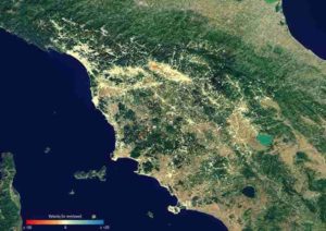
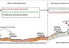
Ground deformation map of the Tuscany region in Italy. Using data acquired between 2014 and 2019 from the Copernicus Sentinel-1 mission, this map shows subsidence in red and uplift in blue. This information is routinely sent to the local authorities in charge of geohazard management practices. The subsidence values derived from the radar data have been overlaid on top of a Copernicus Sentinel-2 image. Credit: contains modified Copernicus Sentinel data (2014-19), processed by ESA/TRE ALTAMIRA
The monitoring of land subsidence is of vital importance for low-lying countries, but also areas which are prone to peculiar ground instability.
Land subsidence is the lowering or sinking of the ground’s surface, owing to changes that take place underground. Subsidence is usually due to a combination of ground water overexploitation, mining, natural consolidation of sediments and rapid urbanization.
This is a major threat, in both urban and agricultural areas, where the continuous lowering over time can cause damage to buildings, sink houses, crack roads, and can cause severe impacts on the environment and economy. In order to support urban development projects and risk assessment efforts, subsidence monitoring is necessary.
Along with the Veneto and Emilia Romagna regions in Italy, Tuscany is an interesting area to analyze, seeing as several cities such as Pistoia, are affected by land subsidence.
Conventional techniques to track and monitor this silent hazard, including repeat optical leveling and groundwater monitoring, can be difficult to manage in the long-term. By using radar data acquired by the Copernicus Sentinel-1 mission over time, ground deformation maps can be created in order to provide a regional monitoring system.
These maps can be useful to analyze past displacement phenomena of a single point in Tuscany over the last few years, in order to help spot unstable areas. This information is routinely sent to the local authorities in charge of geohazard management practices.
The project was driven by the University of Florence, representing the Italian Civil Protection Department, the Regional Government of Tuscany and TRE ALTAMIRA, a company which provides displacement measurements and mapping solutions from satellite radar data at a global level.
Alessandro Ferretti, CEO of TRE ALTAMIRA, comments, “Thanks to Copernicus Sentinel-1, the SAR industry paradigm has definitely changed from ‘mapping’ to ‘monitoring.” Tuscany is the first region in Italy to benefit from this.”
Professor Nicola Casagli from the University of Florence adds, “Satellite data, acquired with short revisiting times and promptly processed, can contribute to the detection of changes in ground deformation patterns, and can feed a decision support system for hydrogeological risk mitigation strategies.”
Radar images—such as those provided by Sentinel-1’s C-band synthetic aperture radar at centimeter precision—are the best way of tracking land subsidence and structural damage across wide areas.
In order to have a continuous flow of displacement information on a regional scale, once a new Copernicus Sentinel-1 image is available, it is automatically downloaded and added to the existing archive. This allows new deformation maps to be generated and updated on a regular basis.
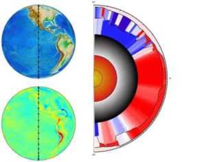
Credit: Density values from LithoRef18 (Afonso et al.) and gravity gradients from Bouman et al. (2016)
A thorough understanding of the ‘solid Earth’ system is essential for deciphering the links between processes occurring deep inside Earth and those occurring nearer the surface that lead to seismic activity such as earthquakes and volcanic eruptions, the rise of mountains and the location of underground natural resources. Thanks to gravity and magnetic data from satellites along with seismology, scientists are on the way to modelling inner Earth in 3-D.
Solid Earth refers to the crust, mantle and core. Because these parts of our world are completely hidden from view, understanding what is going on deep below our feet can only be done by using indirect measurements.
New results, based on a paper published recently in Geophysical Journal International and presented at this week’s Living Planet Symposium, reveal how scientists are using a range of different measurements including satellite data along with seismological models to start producing a global 3-D Earth reference model.
The model will make a step change in being able to analyze Earth’s lithosphere, which is the rigid outer shell, and the underlying mantle to understand the link between Earth’s structure and the dynamic processes within.
Juan Carlos Afonso, from Australia’s Macquarie University and Norway’s Centre for Earth Evolution and Dynamics, said, “We are realising the new global model of Earth’s lithosphere and upper mantle by combining gravity anomalies, geoid height, and gravity gradients complemented with seismic, thermal, and rock information.”
Wolfgang Szwillus from Kiel University, added, “Data from ESA’s GOCE satellite mission served as input for the inversion. It is the first time that gravity gradients have been inverted on a global scale in such an integrated framework.”
While this is just a first step, 3-D Earth offers tantalizing insights into the deep structure of our world. For example, the new models of the thickness of the crust and the lithosphere are important for unexplored continents like Antarctica.
Jörg Ebbing from Kiel University, noted, “This is just a first step so we have more work to do, but we plan to release the 3-D Earth models in 2020.”
The 3-D Earth research, which involves scientists from nine institutes in six European countries, is funded through ESA’s Science for Society programme. ESA’s GOCE gravity mission and Swarm magnetic field mission are key to this research.
Reference:
Juan Carlos Afonso et al. A global reference model of the lithosphere and upper mantle from joint inversion and analysis of multiple data sets, Geophysical Journal International (2019). DOI: 10.1093/gji/ggz094
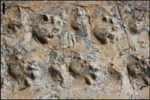
Close-up view of the Ichniotherium trackway from Grand Canyon National Park. Credit: Heitor Francischini
An international team of paleontologists has united to study important fossil footprints recently discovered in a remote location within Grand Canyon National Park, Arizona. A large sandstone boulder contains several exceptionally well-preserved trackways of primitive tetrapods (four-footed animals) which inhabited an ancient desert environment. The 280-million-year-old fossil tracks date to almost the beginning of the Permian Period, prior to the appearance of the earliest dinosaurs.
The first scientific article reporting fossil tracks from the Grand Canyon was published in 1918, just a year before the park was established as a unit of the National Park Service. One hundred years later, during the Centennial Celebration for Grand Canyon National Park, new research on ancient footprints from the park is being presented in a scientific publication released this week. Brazilian paleontologist Dr. Heitor Francischini, from the Laboratory of Vertebrate Paleontology,Federal University of Rio Grande do Sul, is the lead author of the new publication, working with scientists from Germany and the United States.
Francischini and Dr. Spencer Lucas, Curator of Paleontology at the New Mexico Museum of Natural History & Science in Albuquerque, New Mexico, first visited the Grand Canyon fossil track locality in 2017. The paleontologists immediately recognized the fossil tracks were produced by a long-extinct relative of very early reptiles and were similar to tracks known from Europe referred to as Ichniotherium (ICK-nee-oh-thay-ree-um). This new discovery at Grand Canyon is the first occurrence of Ichniotherium from the Coconino Sandstone and from a desert environment. In addition, these tracks represent the geologically youngest record of this fossil track type from anywhere in the world.
Ichniotherium is a kind of footprint believed to have been made by an enigmatic group of extinct tetrapods known as the diadectomorphs. The diadectomorphs were a primitive group of tetrapods that possessed characteristics of both amphibians and reptiles. The evolutionary relationships and paleobiology of diadectomorphs have long been important and unresolved questions in the science of vertebrate paleontology.
Although the actual track maker for the Grand Canyon footprints may never be known for certain, the Grand Canyon trackways preserve the travel of a very early terrestrial vertebrate. The measurable characteristics of the tracks and trackways indicate a primitive animal with short legs and a massive body. The creature walked on all four legs and each foot possessed five clawless digits.
Another interesting aspect of the new Grand Canyon fossil tracks is the geologic formation in which they are preserved. The Coconino Sandstone is an eolian (wind-deposited) rock formation that exhibits cross-bedding and other sedimentary features indicating a desert / dune environment of deposition. Therefore, the presence of Ichniotherium in the Coconino Sandstone is the earliest evidence of diadectomorphs occupying an arid desert environment.
According to Francischini, “These new fossil tracks discovered in Grand Canyon National Park provide important information about the paleobiology of the diadectomorphs. The diadectomorphs were not expected to live in an arid desert environment, because they supposedly did not have the classic adaptations for being completely independent of water. The group of animals that have such adaptations is named Amniota (extant reptiles, birds and mammals) and diadectomorphs are not one of them.”
Lucas also notes that “paleontologists have long thought that only amniotes could live in the dray and harsh Permian deserts. This discovery shows that tetrapods other than reptiles were living in those deserts, and, surprisingly, were already adapted to life in an environment of limited water.”
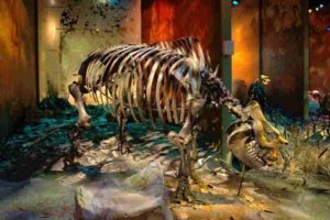
The cast of “Little Guy” mounted on display in the East Tennessee State University Museum of Natural History at the Gray Fossil Site. Credit: Dr. Steven Wallace
Rhinoceros don’t roam the prairies of Texas today, and some might not even know they once roamed the Great Plains. But one Texas A&M University student knows about rhinos: she’s identified unique specimens from fossilized remains found in the mountains of Tennessee dating back almost 5 million years.
Rachel Short, a doctoral candidate in the department of ecosystem science and management at Texas A&M University, is part of a team that identified a new species of ancient rhinoceros, Teleoceras aepysoma, from the late Hemphillian-aged Gray Fossil Site of eastern Tennessee.
The genus, Teleoceras, has been described as the “pot-bellied rhinos,” though this new, taller species changes that, and the species name, aepysoma, means “high-bodied,” Short said. Longer front legs and the lack of a nasal horn are only a few of the body features that make this rhino different from other species already identified.
Short recently published her findings with co-authors Laura Emmert with the Don Sundquist Center of Excellence in Paleontology, and Dr. Steven Wallace, professor and curator of the Museum of Natural History, both at East Tennessee State University.
Short and Emmert completed their master’s degrees at East Tennessee in 2013, and Wallace was their advisor. Short said she got involved with the project because of an interest in North American rhinoceroses that started when she interned at Ashfall Fossil Beds State Historical Park in northeastern Nebraska.
According to the new rhino research, the occurrence of Teleoceras aepysoma in the Appalachian Mountains is unique within a genus typically found in the Great Plains.
“Habitat is most likely a major factor in the unique features,” she said. “We suspect the longer forelimbs helped the rhinos browse on shrubs and trees in the oak-hickory forest. It was a forested environment with little grass, and the smaller tapirs would have been browsing on shorter shrubs, so the rhinos would have had to raise their heads higher.”
Short said it was upon the completion of that project and her interest in the unique morphology and habitat of the Gray Fossil Site rhinos that led her to develop questions that turned in to her Texas A&M dissertation.
At Texas A&M, Short works with Dr. Michelle Lawing to investigate trait-environment relationships of hoofed mammals using bones in the ankle and elbow. The shape of these bones is directly tied to the environment in which the animals live, so fossils can be used to understand past environments as well as how animals respond to environmental change.
“We know mammal communities are being severely impacted by environmental changes,” she said. “We can better predict responses to these ongoing changes if we understand the responses that have been preserved in the information-rich fossil record.”
Teleoceras is a widespread Miocene rhinoceros that has been reported in North American faunas from approximately 20 million years ago to approximately 5 million years ago. The Gray Fossil Site represents one of the last known populations of North American rhinoceroses.
In 2000, late Miocene fossils were found during road construction near Gray, Tennessee, and the Gray Fossil Site was established at the location. There, the fossil material at the site is found primarily in an organic-rich clay deposit that filled a large sinkhole. This sinkhole once served as a watering hole for local fauna, including tapirs, red pandas, alligators and turtles, she said.
Fossils from a minimum of six rhinoceroses, including two nearly complete, articulated skeletons, have been unearthed, Short said, and while Wallace knew they were different, they weren’t studied until she started her master’s thesis in 2011. Availability of such complete specimens enabled a thorough bone-by-bone description of the new species.
Excavations are still ongoing, and as more material is uncovered, the understanding of this unique fauna will improve, she said.
The crystal skulls are human skull hardstone carvings made of clear or milky white quartz, claimed by their alleged finders to be pre-Colombian Mesoamerican artifacts ; however, these claims were refuted for all the specimens available for scientific studies.
The type of crystal was determined by examining chlorite inclusions. It is found only in Madagascar and Brazil, and therefore in pre-Columbian Mesoamerica unrecognizable or unknown.The study concluded that the skulls were made in Germany in the 19th century, most likely at workshops in the city of Idar-Oberstein, renowned in the late 19th century for crafting objects made of imported Brazilian quartz.
There are no uncommon or terribly mysterious crystal skulls. In Brazil, China, and Germany, thousands are produced each year. But a handful of these rather macabre objects have fuelled intense interest and controversy for more than a century among archeologists, scientists, spiritualists, and museum officials.
In private and public collections, there may be a dozen of these rare crystal skulls. Some are crystal-clear, others are quartz smoky or colored. Some of them are of real human size and very fine detail, while others are smaller and less refined. Everyone is supposed to come from Mexico and Central America.
All Fakes?
Moreover, recent analyzes of the British Museum and the Smithsonian Institution’s electron microscope of skulls revealed markings that could only have been made using modern carving tools. Both museums estimate that their skulls date from the mid to late 1800s, a time when there was high public interest in ancient cultures and museums were eager to display pieces.
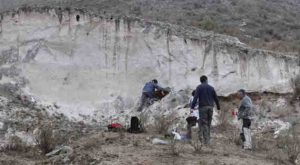
Field work conducted in Tafí del Valle (Tucumán, Argentina)on the ash deposits originated in the Cerro Blanco eruption. Credit: José Luis Fernández-Turiel
Cerro Blanco Volcanic Complex, located in the south of the Altiplano-Puna plateau, erupted around 4,200 years ago. But it was not an ordinary event. It was the largest eruption of the last 5,000 years in the Central Volcanic Zone of the Andes according to a new study published in the journal Estudios Geológicos. The estimated volume of ejected ash places this eruption amongst the largest eruptions of the Holocene Era (the last 11,700 years).
The research team was led by José Luis Fernández Turiel, researcher at Institute of Earth Sciences Jaume Almera of the CSIC (ICTJA-CSIC). Spanish researchers from the University of Las Palmas de Gran Canaria and the Institute of Natural Resources and Agrobiology of Salamanca of the CSIC also participated in the study. They worked alongside Argentinian researchers from the National University of Mar del Plata, the National University of Tucumán and the University of Buenos Aires.
The authors of the study determined that the Cerro Blanco Volcanic Complex, located in the Argentine province of Catamarca, was the source of the thick, high-volume volcanic ash-fall deposits that are still present today in a large area of north-western Argentina. The existence of these deposits was previously known, but not their origin.
Researchers studied 62 outcrops in the area and collected more than 230 ash samples during several field campaigns. In order to determine the origin of these ash deposits, the samples were analysed and characterized by different petrological and geochemical techniques.
“Now we can confirm that the eruption of Cerro Blanco volcano was the event that produced those large Holocene ash deposits that blanketed and cover a large area of the Puna and neighbouring areas of northwestern Argentina,” says José Luis Fernández Turiel, leading author of the study.
The vegetal remains preserved in the sediment layers embedded below the ash deposits were dated using carbon 14. Researchers were able to establish that the eruption took place 4,200 years ago. They reconstructed the transport and the fall of the ash that created the deposits. The eruption of Cerro Blanco was so explosive that the ash was scattered over an area of about 500,000 square kilometres. Ash deposits originated by the eruption were identified and found 400 kilometres away from the volcano caldera, near the town of Santiago del Estero.
In addition, pyroclastic flows filled up the surrounding valleys with thick ignimbrite deposits, some of them located about 35 kilometres away from Cerro Blanco volcano. The emptying of the magmatic chamber caused by the eruption led to the collapse of the volcanic building and the formation of a complex volcanic caldera.
“The geodynamic context of the area determines large explosive eruptions. These are a type of eruptions characterized by rhyolitic magma, with high silica and gas content,” says Francisco José Pérez Torrado, researcher at the Institute of Environmental Studies and Natural Resources of the University of Las Palmas de Gran Canaria.
According to Perez Torrado, “the eruption was not annular, following the edge of the caldera; in this case it was focused on a point to the edge. It was an explosive eruption that pushed an ash and gas cloud at an altitude of almost 32 kilometres according to our simulations.”
According to the study, the volume of deposited ash in this eruption was bigger than 170 cubic kilometres which lead to the researchers to estimate that the eruption of Cerro Blanco had a Volcanic Explosivity Index (VEI) of 7. This places the Cerro Blanco eruption among the largest volcanic global events of the last 10,000 years: it is similar to the eruption that occurred in the Island of Santorini which meant the end of the Minoan civilization. Moreover the volume of magma ejected by Cerro Blanco volcano eruption doubled to the magma ejected by the eruption of the Tambora volcano in 1815, which is thought to be the cause of a global cooling (1815 is known as “the year without summer”).
The present study takes its origin from a previous project conducted to determine whether the high arsenic levels in the water of the Chaco-Pampeana Plain was related to ash-fall deposits of the Central and Southern Andes Volcanic Zones. It was during this work when the team of researchers began to characterize the ashes.
“We verified that the ash from the analysed deposits in the north came mainly from a single eruption, unlike in the south, which clearly came from different volcanoes,” recalls Alejandro Rodríguez González, from the Institute of Environmental Studies and Natural Resources of the University of Las Palmas de Gran Canaria.
According to Fernández-Turiel, “our investigation changes the model of active volcanism of the Central Andean Volcanic Zone. Until now, it was thought that volcanism worked exactly the same, like in the south: many volcanoes with many eruptions over time. What we have seen in our research is that there are few eruptions, but highly explosive and erupting large volumes of magma.”
These findings offer researchers an excellent temporal milestone to study many geological, archaeological and paleoclimatic features, among others, which occurred around the middle Holocene in a broad geographical area of South America.
According to Norma Ratto, archaeologist at the Institute of Cultures of the University of Buenos Aires and CONICET (UBA-CONICET), “the determination of the scope and occurrence of this large eruption provides new information to interpret different aspects of hunter-gatherer societies which inhabited north-western Argentina during the Holocene, as the different occupation of the spaces, the changes in the mobility of the groups due to modification and alteration of routes that allowed the connection between different ecological environments, the changes in the ecosystems and the health of the prehispanic populations, among others topics.”
Reference:
Fernandez-Turiel, J.L., et al. The large eruption 4.2 ks cal BP in Cerro Blanco, Central Volcanic Zone Andes: Insights to the Holocene eruptive deposits in the southern Puna and adjacent regions. 2019. Estudios Geológicos,75 (1): e088 doi.org/10.3989/egeol.43438.515
UNLV geoscientist Terry Spell and former master’s student Dawn Reynoso are part of a research team that discovered primitive monkey teeth in Kenya. The fossils were determined to belong to a previously undiscovered species — filling a 6-million-year void in primate evolution. Credit: Terry Spell/UNLV
Researchers have used fossilized teeth found near Lake Turkana in northwest Kenya to identify a new monkey species—a discovery that helps fill a 6-million-year gap in primate evolution.
UNLV geoscientist Terry Spell and former master’s student Dawn Reynoso were part of the international research team that discovered the species that lived 22 million years ago. Understanding the evolution of Old World monkeys is important because, along with the great apes and humans, they belong to the anthropoid group of primates—primates that resemble humans.
According to Spell, the monkey fossil discovery grew out of a more extensive study of a section of sedimentary rocks in Kenya that contain a large number of different types of fossils, including several hundred mammal and reptile jaws, limbs, and teeth.
Previous studies had documented the early evolution of Old World monkeys using fossils dated at 19 million and 25 million years old, leaving a 6-million-year gap in the earliest record. However, the new fossil was determined to be 22 million years in age. Isotopic ages on the rocks were obtained in the Nevada Isotope Geochronology Laboratory on the UNLV campus.
“This adds to our understanding of the earliest evolutionary history of Old World monkeys, including changes in their diet with time to include more leaves,” Spell said. “Monkeys originated at a time in the past when Africa and Arabia were together as an island continent. Plate tectonic motions pushed this land mass into the Eurasian land mass at 20 to 24 million years ago, and an exchange of animals and plants occurred. It is unclear if competition with newly introduced species or changing climate conditions drove changes in diet.”
Scientists named the newly discovered monkey species Alophia (“without lophs”) due to the lack of molar crests on its teeth—a phenomenon that sets them apart from geologically younger monkey fossils.
Old World monkeys are the most successful living superfamily of nonhuman primates with a geographic distribution that is surpassed only by humans. The group occupies a wide spectrum of land to tree habitats and have a diverse range of diets. They evolved to develop a signature dental feature—having two molar crests—which to this day allows them to process a wide range of food types found in the varying environments of Africa and Asia.
“Primitive Old World monkey from the earliest Miocene of Kenya and the evolution of cercopithecoid bilophodonty” was published in Proceedings of the National Academy of Sciences.
Reference:
D. Tab Rasmussen et al, Primitive Old World monkey from the earliest Miocene of Kenya and the evolution of cercopithecoid bilophodonty, Proceedings of the National Academy of Sciences (2019). DOI: 10.1073/pnas.1815423116
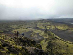
The Laki volcano in Iceland. It is not a typical mountain and its fissure to the right stretches into the distance. Credit: Alan Robock/Rutgers University-New Brunswick
An enormous volcanic eruption on Iceland in 1783-84 did not cause an extreme summer heat wave in Europe. But, as Benjamin Franklin speculated, the eruption triggered an unusually cold winter, according to a Rutgers-led study.
The study, in the Journal of Geophysical Research: Atmospheres, will help improve predictions of how the climate will respond to future high-latitude volcanic eruptions.
The eight-month eruption of the Laki volcano, beginning in June 1783, was the largest high-latitude eruption in the last 1,000 years. It injected about six times as much sulfur dioxide into the upper atmosphere as the 1883 Krakatau or 1991 Pinatubo eruptions, according to co-author Alan Robock, a Distinguished Professor in the Department of Environmental Sciences at Rutgers University–New Brunswick.
The eruption coincided with unusual weather across Europe. The summer was unusually warm with July temperatures more than 5 degrees Fahrenheit above the norm, leading to societal disruption and failed harvests. The 1783–84 European winter was up to 5 degrees colder than average.
Franklin, the U.S. ambassador to France, speculated on the causes in a 1784 paper, the first publication in English on the potential impacts of a volcanic eruption on the climate.
To determine whether Franklin and other researchers were right, the Rutgers-led team performed 80 simulations with a state-of-the-art climate model from the National Center for Atmospheric Research. The computer model included weather during the eruption and compared the ensuing climate with and without the effects of the eruption.
“It turned out, to our surprise, that the warm summer was not caused by the eruption,” Robock said. “Instead, it was just natural variability in the climate system. It would have been even warmer without the eruption. The cold winter would be expected after such an eruption.”
The warm 1783 summer stemmed from unusually high pressure over Northern Europe that caused cold polar air to bypass the region, the study says. After the eruption, precipitation in Africa and Asia dropped substantially, causing widespread drought and famine. The eruption also increased the chances of El Niño, featuring unusually warm water in the tropical Pacific Ocean, in the next winter.
The eruption spawned a sulfuric aerosol cloud – called the “Laki haze” – that lingered over most of the Northern Hemisphere in 1783. Reports from across Europe included lower visibility and the smell of sulfur or hydrogen sulfide. The air pollution was linked to reports of headaches, respiratory issues and asthma attacks, along with acid rain damage to trees and crops, the study notes.
More than 60 percent of Iceland’s livestock died within a year, and about 20 percent of the people died in a famine. Reports of increased death rates and/or respiratory disorders crisscrossed Europe.
“Understanding the causes of these climate anomalies is important not only for historical purposes, but also for understanding and predicting possible climate responses to future high-latitude volcanic eruptions,” Robock said. “Our work tells us that even with a large eruption like Laki, it will be impossible to predict very local climate impacts because of the chaotic nature of the atmosphere.”
Scientists continue to work on the potential impacts of volcanic eruptions on people through the Volcanic Impacts on Climate and Society project. The Laki eruption will be included in their research. Volcanic eruptions can have global climate impacts lasting several years.
The study’s lead author is Brian Zambri, a former post-doctoral associate who earned his doctorate at Rutgers and is now at the Massachusetts Institute of Technology. Scientists at the National Center for Atmospheric Research and University of Cambridge contributed to the study.
Reference:
Brian Zambri et al, Modeling the 1783–1784 Laki Eruption in Iceland, Part II: Climate Impacts, Journal of Geophysical Research: Atmospheres (2019). DOI: 10.1029/2018JD029554
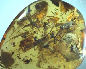
Amber piece showing most large inclusions Credit: NIGPAS
Most amber inclusions are organisms that lived in the forest. It is very rare to find sea life trapped in amber. However, an international research group led by Prof. Wang Bo from the Nanjing Institute of Geology and Palaeontology of the Chinese Academy of Sciences (NIGPAS) reported the first known ammonite trapped in amber in a study in PNAS published on May 13.
The ammonite, a kind of sea animal, was trapped in 99-million-year-old amber from northern Myanmar. The amber is 33 mm long, 9.5 mm wide, 29 mm high and weighs 6.08 g. Besides the ammonite, the amber also encases a diverse assemblage of organisms that today live on land or in the sea, including at least 40 individual animals.
Of the terrestrial fauna found in the amber, mites are the most abundant. Also present are spiders, millipedes, cockroaches, beetles, flies and wasps, most of which would have lived on the forest floor.
Of the marine fauna, in addition to the ammonite itself, sea snails and sea slaters are present. The slaters are like those living on the seashore today.
The researchers used X-ray micro-computed tomography (micro-CT) to obtain high-resolution three-dimensional images of the ammonite including its convoluted sutures, which are important for identifying ammonites.
They found that the ammonite is a juvenile Puzosia (Bhimaites) and its presence in the amber supports a late Albian-early Cenomanian age for the amber deposit. This discovery represents a rare example of dating using amber inclusions.
But how on earth did the ammonite, an extinct sea-dwelling relative of squid, get preserved in a piece of amber that also contains land-based animals? The ammonite and sea snail shells offer possible clues.
The shells are all empty with no soft-tissue, so the organisms were long dead by the time they were engulfed by resin. The outer shell of the ammonite is broken away and the entrance of the shell is full of sand. The amber also contains additional sand.
The most likely explanation for the appearance of both marine and terrestrial organisms within the amber is that a sandy beach covered with shells was located close to resin-producing trees. The flying insects were trapped in the resin while it was still on the tree. As the resin flowed down the tree trunk, it trapped organisms that lived near the foot of the tree. Reaching the beach, it entombed shells and trapped the slaters living there.
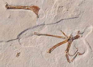
The illustration shows the wing of Alcmonavis poeschli as it was found in the limestone slab. Alcmonavis poeschli is the second known specimen of a volant bird from the Jurassic period.
Archaeopteryx’s throne is tottering. Since the discovery of the first fossil of the primal bird in 1861, it had been considered the only bird from the Jurassic geological period. Today’s birds are thought to be direct descendants of carnivorous dinosaurs, with Archaeopteryx representing the oldest known flying representative of this lineage. All of the specimens that have been found up to now come from the region of the Solnhofen Archipelago, which during the Jurassic era spanned across what is today the Altmühl Valley, in the area between Pappenheim and Regensburg. Archaeopteryx lived here in a landscape of reef islands about 150 million years ago.
A team led by Professor Oliver Rauhut has taxonomically identified a bird unknown until now: Alcmonavis poeschli, the second bird from the era identified as capable of flight. “This suggests that the diversity of birds in the late Jurassic era was greater than previously thought,” says Rauhut, paleontologist at the Department of Earth and Environmental Sciences as well as the Bavarian State Collection of Paleontology and Geology.
Only a wing of Alcmonavis poeschli was discovered. “At first, we assumed that this was another specimen of Archaeopteryx. There are similarities, but after detailed comparisons with Archaeopteryx and other, geologically younger birds, its fossil remains suggested that we were dealing with a somewhat more derived bird,” says Rauhut. According to the team’s taxonomic studies, which are currently featured in the scientific journal eLife, Alcmonavis poeschli was not merely somewhat larger than Archaeopteryx; apparently it could also fly better. “The wing muscles indicate a greater capacity for flying,” says Rauhut. Alcmonavis poeschli exhibits numerous traits lacking in Archaeopteryx but present in more recent birds. This suggests that it was adapted better to active, flapping flight.
The discovery of Alcmonavis poeschli has implications for the debate over whether active flapping birds arose from gliding birds. “Its adaptation shows that the evolution of flight must have progressed relatively quickly,” says Dr. Christian Foth from the University of Fribourg (Switzerland), one of the co-authors of the study.
The bird now being described for the first time derives its name from the old Celtic word for the river Altmühl, Alcmona, and its discoverer Roland Pöschl, who leads the excavation at the Schaudiberg quarry close to Mörnsheim. A fossil of Archaeopteryx was also discovered in the same unit of limestones. The two primal birds thus apparently lived at the same time in what was then a subtropical lagoon landscape in southern Germany.
Reference:
Oliver WM Rauhut, Helmut Tischlinger, Christian Foth. A non-archaeopterygid avialan theropod from the Late Jurassic of southern Germany. eLife, 2019; 8 DOI: 10.7554/eLife.43789
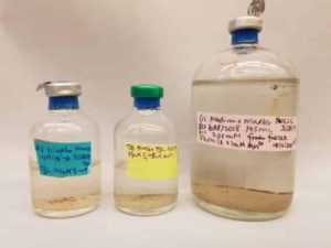
Fine grains of dolomite form on anaerobic microbial mats under various environmental conditions. Credit: Lauren Hinkel
When it comes to making a lasting impression in geological history, the medium makes all the difference, especially in the Earth’s paleo-oceans. Here, during the Archean Eon (4,000-2,500 million years ago) and at times during the Proterozoic (2,500-541 million years ago), when oxygen in the atmosphere and oceans was much lower than today, sedimentary minerals preserved signatures of biological activity in the form of fine textures created by microbial communities. The environmental conditions under which rocks like these form dictate how the crystal structure develops—the more orderly and fine-grained, the better the preservation.
Understanding, and better yet, replicating how these ancient minerals grew provides information about Earth’s past environments, and how organisms developed and behaved. One of these fossil-bearing rocks has proven difficult to copy in the lab—until now.
Researchers from MIT and Princeton University have found a way to emulate a part of ancient Earth in the lab by reproducing one of these weathering-resistant, information-carrying minerals, dolomite, whose formation has long perplexed scientists. A close relative to, and which can be created from, minerals that make limestone, dolomite was pervasive in the past; however, researchers rarely find it in modern environments. While it’s created from components commonly found in seawater, there are physical and kinetic barriers preventing the formation of dolomite—layers of carbonate (CO3-2) ions with alternating central atoms of calcium and magnesium. Alternatively, studies have reported protodolomite—a rock with a disordered crystalline structure, occurring only in very salty modern environments—but this mineral does not preserve the same fine microbial textures as its more ordered brother.
“To look for evidence of ancient life and old processes, you have to look at microbial structures. That’s where the information is. Some of that information is preserved in the form of very finely-grained dolomite, which precipitates almost as the microbes grow. It preserves the lamina of these microbial mats,” says Tanja Bosak, associate professor in the MIT Department of Earth, Atmospheric and Planetary Sciences (EAPS) whose lab led the research. Her group uses experimental geobiology to explore modern biogeochemical and sedimentological processes in microbial systems and interpret the record of life on the early Earth. However, “there’s a big problem about the origin of finely-grained dolomite in a lot of microbial structures through time: There was no clear way of making dolomite under Earth’s surface conditions.”
Their results published in the journal Geology report the first creation of ordered dolomite and find that the trick to capturing these textures may be a slurry of manganese ions, seawater, light, and a biofilm of anaerobic, sulfur-metabolizing, photosynthetic microbes in an oxygen-free environment.
The study’s co-authors are former EAPS postdoc Mirna Daye and Associate Professor John Higgins from Princeton University.
Dolomite problem and the importance of order
Since the first identification of dolomite in the 18th century in what is now known as the Dolomite Mountains of Northern Italy, scientists have been stumped by how dolomite forms, and why there is so much ancient dolomite and so little of the mineral in modern times. This issue was dubbed “the dolomite problem.”
Scientists have found that modern dolomite can form in two main ways. It precipitates when shallow, hypersaline seawater is heated, and when limestone encounters magnesium-rich water, like a deep reef that’s invaded by seawater solutions. However, both methods make large crystals that obscure much of the biological information. In modern seawater, however, aragonite and calcite (different crystalline structures of calcium carbonate) are more likely to precipitate out than dolomite. “It’s not hard to make dolomite if you heat up a beaker of seawater to very high temperatures, but you’ll never get it at the Earth’s surface temperature and pressure just on its own,” says Bosak. “It’s really hard to get magnesium into the minerals; it doesn’t really want to go into the crystal lattice.” That’s a portion of the larger picture. Additionally, these mechanisms do not account for mineral variations (manganese or iron-rich dolomite) seen during the Archean and Proterozoic periods that preserved these textures. “You see that seawater is saturated with respect to dolomite, [but] it just doesn’t form, so there’s some kinetic barrier to that.”
It wasn’t until the turn of the 20th century that a Russian microbiologist demonstrated the potential for anaerobic bacteria to cause dolomite to form from minerals in ocean water, a process called biomineralization. Since then, researchers have found that in modern environments, biofilms—containing photosynthetic microbes and the slimy organic matrix that they excrete for their home (exopolymeric substances)—in highly evaporative pools of salty water can provide a surface on which dolomite can nucleate and grow. However, these biofilms are not photosynthetic. In contrast, many microbial structures that were preserved before the rise of oxygen grew in less-salty marine environments and are thought to have been produced by photosynthetic microbial communities. Additionally, the location of ions and microbes thought to be involved in this process likely differed in the past. The past microbes relied on sulfide, hydrogen, or iron ions for photosynthesis. Researchers suspect that more than 2 billion years ago, manganese and iron ions were present higher in the ocean sediments or even the water column. Today, because of the oxygenated atmosphere, they’re buried deeper in sediments where anaerobic conditions can occur. However, the lack of sunlight means that microbial mats don’t grow here, so neither does dolomite.
While the suggestion of microbial involvement was a strong step to solving the dolomite problem, the matters of crystal ordering and formation in the sunlit marine zone, where microbes colonize sediments, were still unresolved.
Reproducing the past
While investigating early sedimentological preservation, the group performed a series of experiments replicating the conditions of these ancient oceans with an anaerobic atmosphere. They used a combination of modern biofilms, light/dark environments, and seawater modified to mimic early Earth conditions with and without manganese, one of the metals often found in the mineral and thought to facilitate bacterial growth. The researchers used microbes from a lake in upstate New York, from depths that lack oxygen.
In their experiments, the researchers noticed something unexpected—that the most abundant mineral in the biofilms was highly ordered dolomite, and the vials that produced the most contained photosynthesizing microbes and manganese—a result consistent with field reports. As the mats grew up toward the light, crystals accumulated on them, with the oldest on the bottom capturing tiny wiggles where now degraded microbial mats used to be. The more extensive the coverage, the smaller the porosity, which reduced the chances of fluids infiltrating them, interacting with and dissolving the minerals, and essentially erasing data. The experiments lacking manganese or performed in the dark (not photosynthesizing) developed disordered dolomite. “We don’t understand exactly why manganese and the microbes have that effect, but it seems like they do. It’s almost like a natural consequence of those types of conditions,” says Bosak. Nonetheless, “It was a big deal to show that that can actually happen.”
Now that the team has found a way to make ordered dolomite, they plan to look into why it forms, variations, and how the rock records the environmental conditions it forms in. After seeing the effect that manganese had on dolomite, the researchers will look at iron ions, which integrated into these ancient rocks. “Iron also seems to stimulate the formation of the incorporation of magnesium into this mineral, for whatever reason,” says Bosak.
They’ll also investigate the unique microbial interactions and physical properties present to see what components are essential to precipitating dolomite. The individual niches that each anaerobic organism occupies seem to help the community grow, cycle elements, degrade substances, and provide a surface for crystals. The Bosak group will do this by fossilizing various organisms under the same or different environmental conditions to see if they can produce dolomite. During these experiments, they will monitor how well dolomite records the temperature at which it was made, as well as the chemical and isotopic composition of the surrounding solution, to understand the process better.
“I think it tells us that—when we are trying to interpret the past—it’s a really different planet: different types of organisms, different types of metabolisms that were dominant,” says Bosak, “and I think we are just starting to scratch the surface of what possible mineral outcomes, what kind of textural outcomes we can even expect.”
Reference:
Mirna Daye et al. Formation of ordered dolomite in anaerobic photosynthetic biofilms, Geology (2019). DOI: 10.1130/G45821.1
It is a diamond with the same mineral properties as colorless diamonds, displaying red color. They are commonly known as the world’s most expensive and rare color of diamonds, more so than pink diamonds or blue diamonds.
It is like pink diamonds, are highly debated as to the source of their color, but the gemological community most frequently attributes both colors to gliding atoms in the structure of the diamond as it undergoes tremendous pressure during its formation.
They are among the twelve colors of fancy diamonds, the most expensive per carat price. They usually run in the range of hundreds of thousands of dollars per carat. Because they are the rarest color, they are hard to find in large sizes and are mostly found in sizes below 1 carat.
It exist only with one intensity of colour, Fancy, although their clarity may vary from Flawless to Included, just like white diamonds. The biggest and most flawless red diamond is the Red Diamond 5.11 carat Fancy Red Moussaieff, which has flawless clarity internally.
Source of Red Color in Diamonds
The most widely accepted theory is that a plastic deformation is caused in the crystal lattice structure during the formation of the diamond. Some of the atoms are misplaced as the diamond moves through its deposit of kimberlite, and this movement’s intense pressure causes the different shades of pink or red to appear.
This credits the hypothesis that they are actually extremely dark pink diamonds and why only one intensity of color is possible. It can be modified by the same secondary colors that can also be found to modify pink diamonds.
Red color can be produced with high-energy particles irradiating a colorless diamond and then annealing it at high pressures and high temperatures.
Where Can Red Diamond be Found?
Red diamond source mines. Most of the them mined each year come from Kimberley, Western Australia’s Argyle diamond mine. They were also found in Brazil, Russia, and some African countries, though.
How Much Red Diamond?
In 1987, the first gem quality called the Hancock Red sold for over $926,000 per carat!
“Pure” red diamonds are so rare and disproportionately priced that they are generally beyond the scope of celebrity life and are rarely found above 1 Carat. As an example, this SI2 Clarity grade 0.71 Carat Fancy Red Diamond Radiant is priced at $ 603,600!
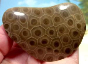
A Petoskey Stone is a rock and a fossil composed of a fossilized rugose coral, Hexagonaria percarinata, which is often pebble-shaped. Such stones were formed as a result of glaciation, where sheets of ice plucked stones from the bedrock, grinding off their rough edges and depositing them in the lower peninsula of Michigan’s northwest (and some in the northeast). Complete fossilized coral heads can be found in the source rocks for the Petoskey stones in the same areas of Michigan.
Petoskey stones are found in the Traverse Group’s Gravel Point Formation. They are fragments of an originally deposited coral reef during the Devonian period. When dry, the stone resembles ordinary calcareous but the distinctive mottled pattern of six-sided coral fossils emerges when wet or polished using lapidary techniques. It is sometimes turned into objects of decoration. There are also other forms of fossilized coral in the same location.
It was named Michigan’s state stone in 1965.
Where Is Petoskey Stone Found?
Petoskey stones can be found in Michigan on different beaches and inland locations, with many of the most popular being those around Petoskey and Charlevoix. During the winters, the frozen lake ice movement acting on the shore is thought to turn over stones at the shore of Lake Michigan, exposing new Petoskey stones at the edge of the water every spring.
Also present in the fossil records of Iowa, Indiana, Illinois, Ohio, New York and locations in Canada, Germany, England, and Asia is the type of coral that forms the basis of Petoskey Stones.
Subduction Zone. Credit: California Institute of Technology
It is well known that life on Earth and the geology of the planet are intertwined, but a new study provides fresh evidence for just how deep—literally—that connection goes. Geoscientists at Caltech and UC Berkeley have identified a chemical signature in igneous rocks recording the onset of oxygenation of Earth’s deep oceans—a signal that managed to survive the furnace of the mantle. This oxygenation is of great interest, as it ushered in the modern era of high atmospheric and oceanic oxygen levels, and is believed to have allowed the diversification of life in the sea.
Their findings, which were published in Proceedings of the National Academy of Science on April 11, support a leading theory about the geochemistry of island arc magmas and offer a rare example of biological processes on the planet’s surface affecting the inner Earth.
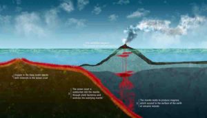
Island arcs are formed when one oceanic tectonic plate slides beneath another in a process called subduction. The subducting plate descends and releases water-rich fluids into the overlying mantle, causing it to melt and produce magmas that ultimately ascend to the surface of the earth. This process builds island arc volcanoes like those found today in the Japanese islands and elsewhere in the Pacific Ring of Fire. Eventually, through plate tectonics, island arcs collide with and are incorporated into continents, preserving them in the rock record over geological time.
The most abundant magmatic, or igneous, rocks are basalts—dark-colored and fine-grained rocks commonly found in lava flows. Most basalts on the earth today do not form at island arcs but rather at mid-ocean ridges deep underwater. A well-known difference between the two is that island arc basalts are more oxidized than those found at mid-ocean ridges.
A leading but debated hypothesis for this difference is that oceanic crust is oxidized by oxygen and sulfate in the deep ocean before it is subducted into the mantle, delivering oxidized material to the mantle source of island arcs above the subduction zone.
But Earth is not thought to have always had an oxygenated atmosphere and deep ocean. Rather, scientists believe, the emergence of oxygen—and with it the ability for the planet to sustain aerobic life—occurred in two steps. The first event, which took place between about 2.3 and 2.4 billion years ago, resulted in a greater than 100,000-fold increase in atmospheric O2 in the atmosphere, to about 1 percent of modern levels.
Although it was dramatically higher than it had previously been, the atmospheric O2 concentration at this time still was too low to oxygenate the deep ocean, which is thought to have remained anoxic until around 400 to 800 million years ago. Around that time, atmospheric O2 concentrations are thought to have increased to 10 to 50 percent of modern levels. That second jump has been proposed to have allowed oxygen to circulate into the deep ocean.
“If the reason why modern island arcs are fairly oxidized is due the presence of dissolved oxygen and sulfate in the deep ocean, then it sets up an interesting potential prediction,” says Daniel Stolper (Caltech Ph.D. ’14), one of the authors of the paper and an assistant professor of Earth and Planetary Science at UC Berkeley. “We know roughly when the deep oceans became oxygenated and thus, if this idea is right, one might see a change in how oxidized ancient island arc rocks were before versus after this oxygenation.”
To search for the signal of this oxygenation event in island arc igneous rocks, Stolper teamed up with Caltech assistant professor of geology Claire Bucholz, who studies modern and ancient arc magmatic rocks. Stolper and Bucholz combed through published records of ancient island arcs and compiled geochemical measurements that revealed the oxidation state of arc rocks that erupted tens of millions to billions of years ago. Their idea was simple: if oxidized material from the surface is subducted and oxidizes the mantle regions that source island arc rocks, then ancient island arc rocks should be less oxidized (and thus more “reduced”) than their modern counterparts.
“It’s not as common anymore, but scientists used to routinely quantify the oxidation state of iron in their rock samples,” Bucholz says. “So there was a wealth of data just waiting to be reexamined.”
Their analysis revealed a distinct signature: a detectable increase in oxidized iron in bulk-rock samples between 800 and 400 million years ago, the same time interval that independent studies proposed the oxygenation of the deep ocean occurred. To be thorough, the researchers also explored other possible explanations for the signal. For example, it is commonly assumed that the oxidation state of iron in bulk rocks can be compromised by metamorphic processes—the heating and compaction of rocks—or by processes that alter them at or near the surface of the earth. Bucholz and Stolper constructed a variety of tests to determine whether such processes had affected the record. Some alteration almost certainly occurred, Bucholz says, but the changes are consistent everywhere that samples were taken. “The amount of oxidized iron in the samples may have been shifted after cooling and solidification, but it appears to have been shifted in a similar way across all samples,” she says.
Stolper and Bucholz additionally compiled another proxy also thought to reflect the oxidation state of the mantle source of arc magmas. Reassuringly, this independent record yielded similar results to the iron-oxidation-state record. Based on this, the researchers propose that the oxygenation of the deep ocean impacted not only on the earth’s surface and oceans but also changed the geochemistry of a major class of igneous rocks.
This work complements earlier research by Bucholz that examines changes in the oxidation signatures of minerals in igneous rocks associated with the first oxygenation event 2.3 billion years ago. She collected sedimentary-type, or S-type, granites, which are formed during the burial and heating of sediments during the collision of two landmasses—for example, in the Himalayas, where the Indian subcontinent is colliding with Asia.
“The granites represent melted sediments that were deposited at the surface of Earth. I wanted to test the idea that sediments might still record the first rise of oxygen on Earth, despite having been heated up and melted to create granite,” she says. “And indeed, it does.”
Both studies speak to the strong connection between the geology of Earth and the life that flourishes on it, she says. “The evolution of the planet and of the life on it are intertwined. We can’t understand one without understanding the other,” says Bucholz.
The PNAS study is titled “Neoproterozoic to early Phanerozoic rise in island arc redox state due to deep ocean oxygenation and increased marine sulfate levels.”
Reference:
Daniel A. Stolper et al. Neoproterozoic to early Phanerozoic rise in island arc redox state due to deep ocean oxygenation and increased marine sulfate levels, Proceedings of the National Academy of Sciences (2019). DOI: 10.1073/pnas.1821847116
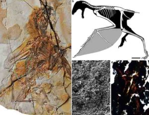
a. Fossil; b. restoration, scale bar equal 10 mm; c. melanosomes of the membranous wing (mw); d. histology of the bony stomach content (bn). st, styliform element; gs, gastroliths Credit: WANG Min
A new Jurassic non-avian theropod dinosaur from 163 million-year-old fossil deposits in northeastern China provides new information regarding the incredible richness of evolutionary experimentation that characterized the origin of flight in the Dinosauria.
Drs. Wang Min, Jingmai K. O’Connor, Xu Xing, and Zhou Zhonghe from the Institute of Vertebrate Paleontology and Paleoanthropology (IVPP) of the Chinese Academy of Sciences described and analyzed the well-preserved skeleton of a new species of Jurassic scansoriopterygid dinosaur with associated feathers and membranous tissues. Their findings were published in Nature.
The new species, named Ambopteryx longibrachium, belongs to the Scansoriopterygidae, one of the most bizarre groups of non-avian theropods. The Scansoriopterygidae differ from other theropods in their body proportions, particularly in the proportions of the forelimb, which supports a bizarre wing structure first recognized in a close relative of Ambopteryx, Yi qi.
Unlike other flying dinosaurs, namely birds, these two species have membranous wings supported by a rod-like wrist bone that is not found in any other dinosaur (but is present in pterosaurs and flying squirrels).
Until the discovery of Yi qi in 2015, such a flight apparatus was completely unknown among theropod dinosaurs. Due to incomplete preservation in the holotype and only known specimen of Yi qi, the veracity of these structures and their exact function remained hotly debated.
As the most completely preserved specimen to date, Ambopteryx preserves membranous wings and the rod-like wrist, supporting the widespread existence of these wing structures in the Scansoriopterygidae.
WANG and his colleagues investigated the ecomorphospace disparity of Ambopteryx relative to other non-avian coelurosaurians and Mesozoic birds. The results showed dramatic changes in wing architecture evolution between the Scansoriopterygidae and the avian lineage, as the two clades diverged and underwent very different evolutionary paths to achieving flight.
Interestingly, forelimb elongation, an important characteristic of flying dinosaurs, was achieved in scansoriopterygids primarily through elongation of the humerus and ulna, whereas the metacarpals were elongated in non-scansoriopterygid dinosaurs including Microraptor and birds.
In scansoriopterygids, the presence of an elongated manual digit III and the rod-like wrist probably compensated for the relatively short metacarpals and provided the main support for the membranous wings. In contrast, selection for relatively elongated metacarpals in most birdlike dinosaurs was likely driven by the need for increased area for the attachment of the flight feathers, which created the wing surface in Microraptor and birds.
The co-occurrence of short metacarpals with membranous wings, versus long metacarpals and feathered wings, exhibits how the evolution of these two significantly different flight strategies affected the overall forelimb structure. So far, all known scansoriopterygids are from the Late Jurassic and their unique membranous wing structure did not survive into the Cretaceous.
This suggests that this wing structure represents a short-lived and unsuccessful attempt to fly. In contrast, feathered wings, first documented in Late Jurassic non-avian dinosaurs, were further refined through the evolution of numerous skeletal and soft tissue modifications, giving rise to at least two additional independent origins of dinosaur flight and ultimately leading to the current success of modern birds.
Reference:
Min Wang et al. A new Jurassic scansoriopterygid and the loss of membranous wings in theropod dinosaurs, Nature (2019). DOI: 10.1038/s41586-019-1137-z
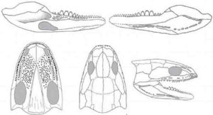
Reconstructed skull and lower jaw of Acherontiscus caledoniae
Micro-CT scanning of a tiny snake-like fossil discovered in Scotland has shed new light on the elusive creature, thought to be one of the earliest known tetrapods to develop teeth that allowed it to crush its prey.
Detailed scans of Acherontiscus caledoniae showed a unique combination of different tooth shapes and sizes as well as a deep lower jaw which scientists believe would have given the creature the ability to pierce, cut and grind the hard-shelled crustaceans that made up its diet.
Scientists led by the University Museum of Zoology in Cambridge alongside the University of Lincoln, the Natural History Museum in London and the University of Southampton, found that the dental pattern of Acherontiscus is at odds with that of several other tetrapods of this period, which tended to have uniform rows of cone-like teeth sometimes curved backwards at the tip. The variation in the shape and size of teeth shown in this fossil displays a level of dental adaptation that is unprecedented in such an early tetrapod.
As co-author Dr Marcello Ruta from the University of Lincoln’s School Of Life Sciences explains: “We found that Acherontiscus preceded the origin of modern tetrapod lineages and joined an array of primitive groups that independently acquired long and often miniaturized bodies, and exhibited either reduced or no limbs.”
The fossil is the only known specimen of this limbless tetrapod, which measured just 6 inches long and existed in swampy marshlands on the outskirts of Edinburgh some 330 million years ago. The delicate nature of the fossil meant that scientists were unable to use mechanical or chemical methods to free its skeleton from the surrounding rock, or study the specimen under a microscope.
Lead author Professor Jennifer Clack from the University Museum of Zoology in Cambridge said: “Using advanced techniques of micro-CT scanning, we were able to make sense of Acherontiscus’ complex skull, revealing minute anatomical details that allowed us to produce a greatly revised and much more complete reconstruction.
“We were particularly surprised to realize the great variety of shapes and sizes of its teeth. Acherontiscus is the earliest known tetrapod showing a crushing dentition, a feature with a rather discontinuous distribution in fossil and modern tetrapods.”
Fragments in the surrounding matrix have also revealed more about Acherontiscus’ habitat which will inform further research into the area as co-author Professor John Marshall from the University of Southampton’s School of Ocean and Earth Science explains: “Our study provided impetus for exploring the ecology and environments of the Scottish wetlands where Acherontiscus lived. Analysis of the content of fossil spores from about 0.2 grams of the matrix surrounding the creature suggests that this animal lived close to or within a still water body surrounded by herbaceous plants related to clubmosses. A more distant forest of larger, tree-like relatives of modern quillworts was also present.”
Reference:
Jennifer A. Clack, Marcello Ruta, Andrew R. Milner, John E. A. Marshall, Timothy R. Smithson, Keturah Z. Smithson. Acherontiscus caledoniae: the earliest heterodont and durophagous tetrapod. Royal Society Open Science, 2019; 6 (5): 182087 DOI: 10.1098/rsos.182087
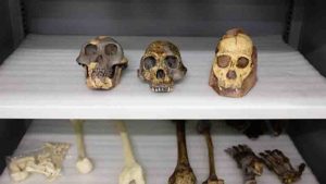
Fossil casts of Australopithecus afarensis (left), Homo habilis (center), and Australopithecus sediba (right)
Statistical analysis of fossil data shows that it is unlikely that Australopithecus sediba, a nearly two-million-year-old, apelike fossil from South Africa, is the direct ancestor of Homo, the genus to which modern-day humans belong.
The research by paleontologists from the University of Chicago, published this week in Science Advances, concludes by suggesting that Australopithecus afarensis, of the famous “Lucy” skeleton, is still the most likely ancestor to the genus Homo.
The first A. sediba fossils were unearthed near Johannesburg in 2008. Hundreds of fragments of the species have since been discovered, all dating to roughly two million years ago. The oldest known Homo fossil, the jawbone of an as yet unnamed species found in Ethiopia, is 2.8 million years old, predating A. sediba by 800,000 years.
Despite this timeline, the researchers who discovered A. sediba have claimed that it is an ancestral species to Homo. While it is possible that A. sediba (the hypothesized ancestor) could have postdated earliest Homo (the hypothesized descendant) by 800,000 years, the new analysis indicates that the probability of finding this chronological pattern is highly unlikely.
“It is definitely possible for an ancestor’s fossil to postdate a descendant’s by a large amount of time,” said the study’s lead author Andrew Du, PhD, who will join the faculty at Colorado State University after concluding his postdoctoral research in the lab of Zeray Alemseged, PhD, the Donald M. Pritzker Professor of Organismal and Biology and Anatomy at UChicago.
“We thought we would take it one step further to ask how likely it is to happen, and our models show that the probability is next to zero,” Du said.
Du and Alemseged also reviewed the scientific literature for other hypothesized ancestor-descendant relationships between two hominin species. Of the 28 instances they found, only one first-discovered fossil of a descendant was older than its proposed ancestor, a pair of Homo species separated by 100,000 years, far less than the 800,000 years separating A. sediba and earliest Homo. For context, the average lifespan of any hominin species is about one million years.
“Again, we see that it’s possible for an ancestor’s fossil to postdate its descendant’s,” Du said. “But 800,000 years is quite a long time.”
Alemseged and Du maintain that Australopithecus afarensisis a better candidate for the direct ancestor of Homofor a number of reasons. A. afarensis fossils have been dated up to three million years old, nearing the age of the first Homo jaw. Lucy and her counterparts, including Selam, the fossil of an A. afarensischild that Alemseged discovered in 2000, were found in Ethiopia, just miles from where the Homo jaw was discovered. The jaw’s features also resemble those of A. afarensis closely enough that one could make the case it was a direct descendant.
“Given the timing, geography and morphology, these three pieces of evidence make us think afarensisis a better candidate than sediba,” Alemseged said. “One can disagree about morphology and the different features of a fossil, but the level of confidence we can put in the mathematical and statistical analyses of the chronological data in this paper makes our argument a very strong one.”
Reference:
Andrew Du and Zeresenay Alemseged. Temporal evidence shows Australopithecus sediba is unlikely to be the ancestor of Homo. Science Advances, 2019 DOI: 10.1126/sciadv.aav9038
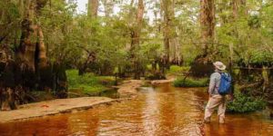
David Stahle in North Carolina’s Black River. Photo by Dan Griffin.
A recently documented stand of bald cypress trees in North Carolina, including one tree at least 2,624 years old, are the oldest known living trees in eastern North America and the oldest known wetland tree species in the world.
David Stahle, Distinguished Professor of geosciences, along with colleagues from the university’s Ancient Bald Cypress Consortium and other conservation groups, discovered the trees in 2017 in a forested wetland preserve along the Black River south of Raleigh, North Carolina. Stahle documented the age of the trees using dendrochronology, the study of tree rings, and radio carbon dating. His findings were published May 9 in the journal Environmental Research Communications.
The ancient trees are part of an intact ecosystem that spans most of the 65-mile length of the Black River. In addition to their age, the trees are a scientifically valuable means of reconstructing ancient climate conditions. The oldest trees in the preserve extend the paleoclimate record in the southeast United States by 900 years, and show evidence of droughts and flooding during colonial and pre-colonial times that exceed any measured in modern times.
“It is exceedingly unusual to see an old-growth stand of trees along the whole length of a river like this,” Stahle said. “Bald cypress are valuable for timber and they have been heavily logged. Way less than 1 percent of the original virgin bald cypress forests have survived.”
Stahle has been working in the area since 1985, and cataloged bald cypress trees as old as 1,700 years in a 1988 study published in the journal Science. His work helped preserve the area, 16,000 acres of which have since been purchased by The Nature Conservancy, a private land-conservation group that keeps most of its holdings open to the public.
“Dr. Stahle’s original work on the Black River, which showed trees dating from Roman times, inspired us to begin conservation on the Black more than two decades ago,” said Katherine Skinner, executive director of The North Carolina Chapter of The Nature Conservancy. “This ancient forest gives us an idea of what much of North Carolina’s coastal plain looked like millennia ago. It is a source of inspiration and an important ecosystem. Without Dr. Stahle, it would have gone unprotected and likely destroyed.”
For the newest study, researchers used non-destructive core samples from 110 trees found in a section of the wetland forest they had not previously visited. “The area of old growth bald cypress was 10 times larger than I realized,” Stahle said. “We think there are older trees out there still.”
Reference:
D W Stahle, J R Edmondson, I M Howard, C R Robbins, R D Griffin, A Carl, C B Hall, D K Stahle, M C A Torbenson. Longevity, climate sensitivity, and conservation status of wetland trees at Black River, North Carolina. Environmental Research Communications, 2019; 1 (4): 041002 DOI: 10.1088/2515-7620/ab0c4a
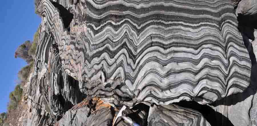
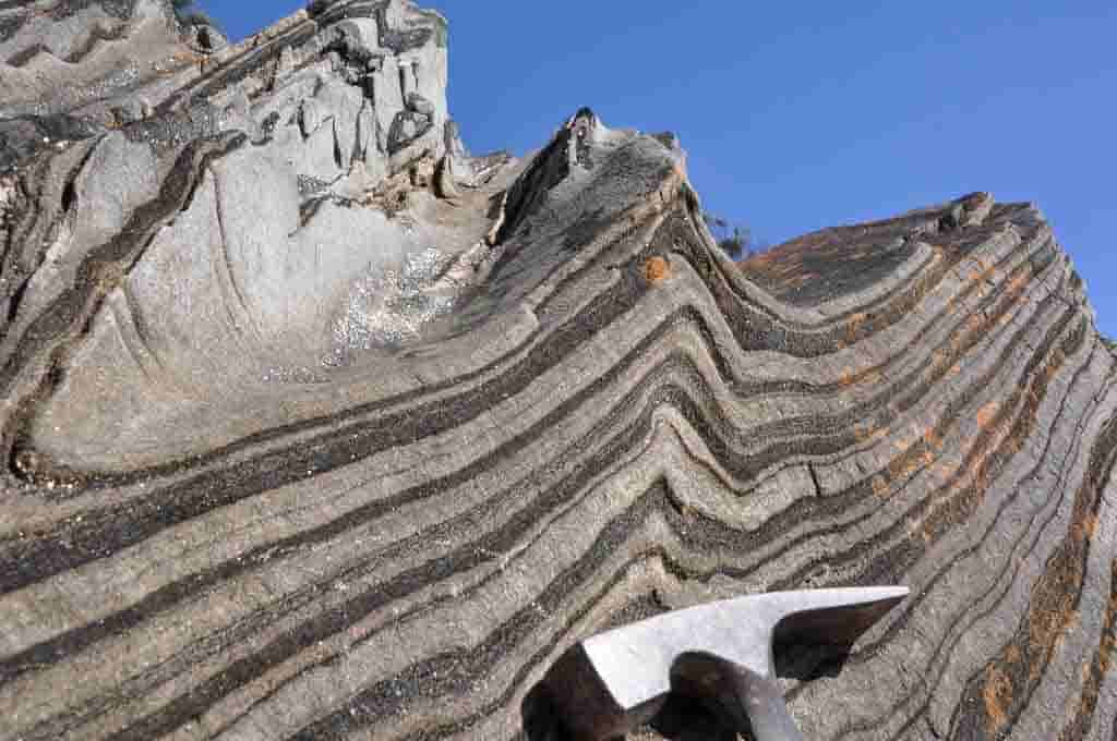
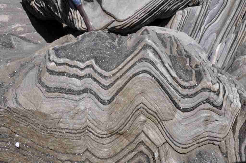
Photographed on Kangaroo Island, this rock – called a ‘zebra schist’ – deformed from flat-lying marine sediments through being stressed by a continental collision over 500 million years ago. Credit: Dietmar Muller, CC BY
Zebra Schist
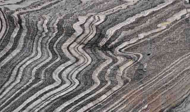
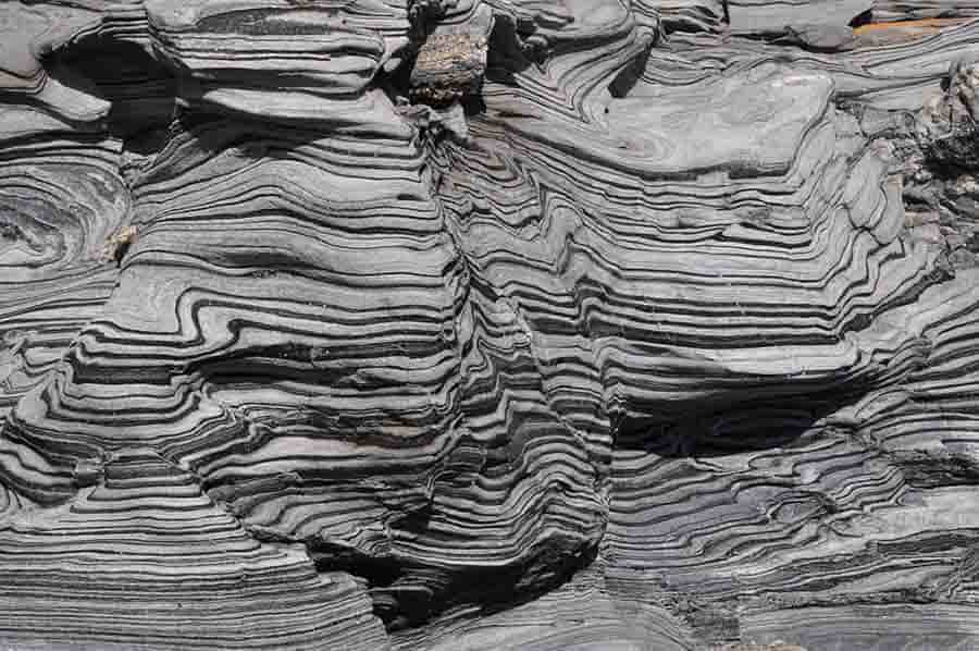
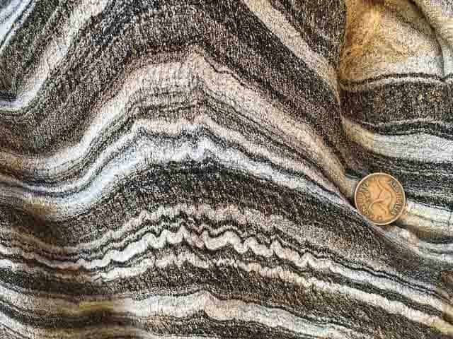
Zebra Schist is The tightly folded, thinly bedded schists that are derived from sedimentary rocks that are exposed in Kangaroo Island are known as zebra schists. A quartz-rich and biotite-rich layering largely reflects original sedimentary layering rather than metamorphic differentiation as the secondary biotite preserves and outlines a variety of sedimentary structures.
Small cross-beds troughs and climbing ripples show a sequence facing south. The Geological Society of Australia
has designated this section of the coastline as a geological monument.
Where is Zebra Schist found?
It Found in Harvey’s Return, Kangaroo Island, South Australia
What is Schist?
Schist is a metamorphic rock of medium grade. In a preferred orientation, Schist has medium to large, flat, sheet-like grains (nearby grains are approximately parallel). It is defined by having platy and elongated minerals (such as micas or talc) of more than 50 percent, often finely interleaved with quartz and feldspar.
These minerals include micas, chlorite, talc, hornblende, graphite, and other lamellar (flat, planar). In drawn-out grains, quartz often occurs to such an extent that a particular shape is produced called quartz schist. Often schist is garnetiferous. At a higher temperature, schist forms and has larger grains than phyllite. Geological foliation with medium to large grained flakes in a preferred sheetlike orientation is called schistosity (metamorphic arrangement in layers).
Zebra Schist
1 of 6
Photographed on Kangaroo Island, this rock – called a ‘zebra schist’ – deformed from flat-lying marine sediments through being stressed by a continental collision over 500 million years ago. Credit: Dietmar Muller, CC BY
Photographed on Kangaroo Island, this rock – called a ‘zebra schist’ – deformed from flat-lying marine sediments through being stressed by a continental collision over 500 million years ago. Credit: Dietmar Muller, CC BY
A new study from The University of Texas at Austin looks at the complex geology that contributed to the 2010 Deepwater Horizon disaster. Credit: US Coast Guard
A study from The University of Texas at Austin is the first published in a scientific journal to take an in-depth look at the challenging geologic conditions faced by the crew of the Deepwater Horizon drilling rig and the role those conditions played in the 2010 disaster.
The well blowout killed 11 people and spewed oil for three months, spilling about 4 million barrels of oil into the Gulf of Mexico before crews successfully capped the well. Researchers and investigators since then have focused mostly on the engineering decisions and mistakes that led to the blowout and the ecological impacts of the oil spill that became one of the country’s worst environmental catastrophes. But researchers from the UT Jackson School of Geosciences, aided by thousands of pages of documents made public during lawsuits and legal proceedings, have pieced together how the geologic conditions more than 2 miles under the Gulf floor made drilling difficult and drove engineering decisions that contributed to the well’s failure and the ensuing blowout.
The study, published May 7 in Scientific Reports, documents, among other things, a significant and steep drop in pore pressure inside the rock near the bottom of the well that influenced the decisions that contributed to the blowout.
“The paper tells the geological story behind the catastrophe,” said Will Pinkston, who authored the paper while earning a master’s degree at the Jackson School. “It is high impact science, and I’m excited to reach a wider audience of people who don’t think about these issues every day.”
The engineering and geosciences challenges posed by drilling wells miles under the surface of the earth are enormously complex. One of the most critical is to maintain the pressure within the well so that it is higher than the pressure within the fluid inside the rock but lower than the stress at which the rock fails. If pressure inside the well is too high, it will fracture the well wall and drive drilling fluids into the rock. If the well pressure is lower than the rock’s fluid pressure, fluids from inside the surrounding rock will flow into the well and potentially cause a blowout.
To successfully drill, crews use drilling “mud,” a slurry that can be mixed to varying weights and consistency, which is circulated throughout the well to help stabilize the hole and control pressure. Crews then line the exposed well with cement and steel casing to seal off exposed rock.
In the case of the Transocean Deepwater Horizon drilling rig, which was operated by the BP energy company at the time of the accident, the pore pressure was very high throughout the well, but then dropped abruptly by about 1,200 pounds per square inch near the bottom. Most of the pore pressure drop occurred in the 100 feet above the reservoir target of 18,000 feet below sea level.
BP planned to temporarily abandon the oil well, the initial well in the Macondo prospect, until it could be produced at a later date, by plugging the base with steel and cement. However, the sharp drop in pore pressure, and an associated decline in stress, drastically narrowed the range of options to seal off the well. This led to the decision to use a controversial low-density foam cement that failed to set properly. This was a key cause of the Macondo well blowout.
“The bottom line is that the geological conditions led to a decision to use a specialized cement that failed,” said Peter Flemings, a Jackson School professor and study author. “This decision was a root cause of the ultimate blowout.”
Flemings was a member of the Deepwater Horizon well integrity team assembled by then-U.S. Energy Secretary Steven Chu to help respond to the disaster.
Beyond describing the pressure and stress conditions in the well, the paper maps geologic conditions across the entire subterranean basin to show that the pressure drop is not a unique event in that area.
“Macondo isn’t a one-dimensional problem,” Pinkston said. “We found evidence of large-scale fluid connectivity across the basin, and this would have been hard to predict.”
Although the paper does not pinpoint any single reason for the catastrophe, Flemings said it offers important information for the larger drilling community.
“One of the significant things about this paper is to get all the data on the table so that the general community can understand the decisions that were made,” Flemings said.
“I broadly believe that if engineers and geoscientists are more aware of how pressure and stress and engineering decisions couple, better decisions will be made.”
The study was funded by Flemings and the UT GeoFluids consortium. Data from the consortium and the University of Texas Institute for Geophysics Gulf Basin Depositional Synthesis project were used in this study. BP is one of the companies that supports the consortium.
Reference:
F. William M. Pinkston, Peter B. Flemings. Overpressure at the Macondo Well and its impact on the Deepwater Horizon blowout. Scientific Reports, 2019; 9 (1) DOI: 10.1038/s41598-019-42496-0