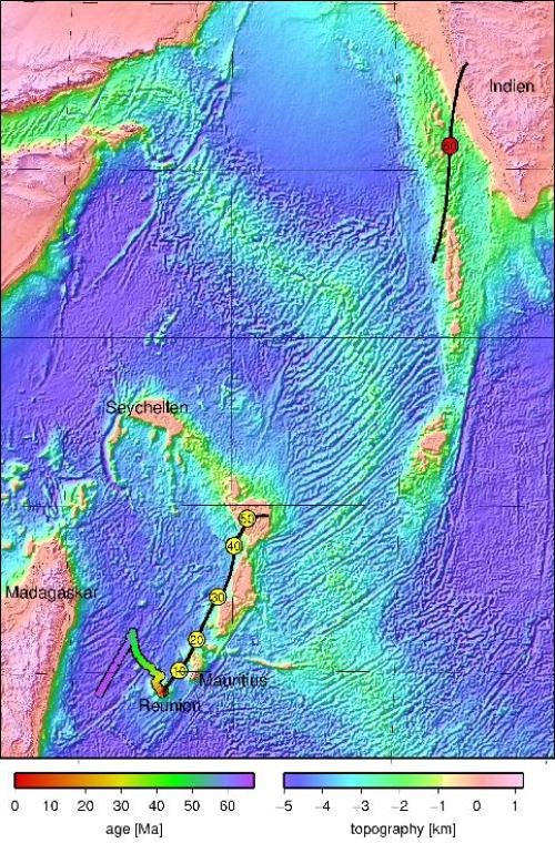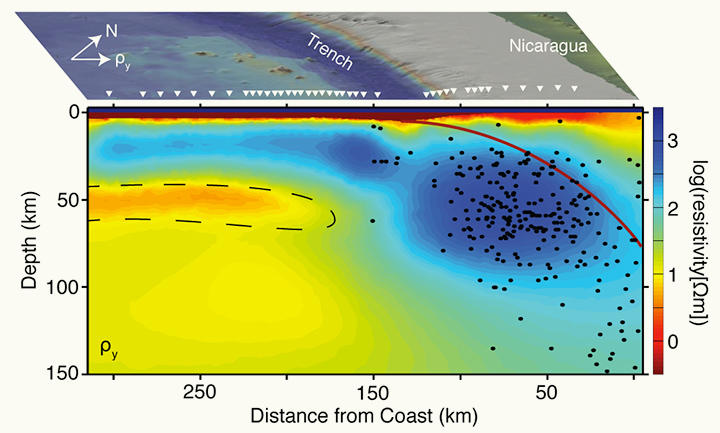
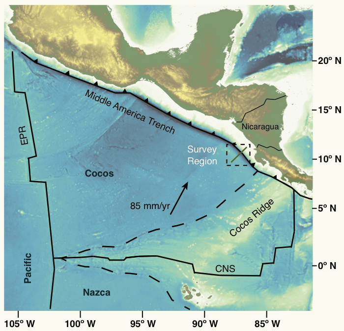
Scientists at Scripps Institution of Oceanography at UC San Diego have found a layer of liquefied molten rock in Earth’s mantle that may be acting as a lubricant for the sliding motions of the planet’s massive tectonic plates. The discovery may carry far-reaching implications, from solving basic geological functions of the planet to a better understanding of volcanism and earthquakes.The scientists discovered the magma layer at the Middle America trench offshore Nicaragua. Using advanced seafloor electromagnetic imaging technology pioneered at Scripps, the scientists imaged a 25-kilometer- (15.5-mile-) thick layer of partially melted mantle rock below the edge of the Cocos plate where it moves underneath Central America.
The discovery is reported in the March 21 issue of the journal Nature by Samer Naif, Kerry Key, and Steven Constable of Scripps, and Rob Evans of Woods Hole Oceanographic Institution.
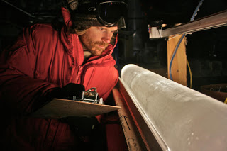
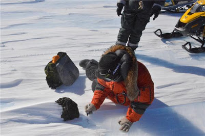
The new images of magma were captured during a 2010 expedition aboard the U.S. Navy-owned and Scripps-operated research vessel Melville. After deploying a vast array of seafloor instruments that recorded natural electromagnetic signals to map features of the crust and mantle, the scientists realized they found magma in a surprising place.
“This was completely unexpected,” said Key, an associate research geophysicist in the Cecil H. and Ida M. Green Institute of Geophysics and Planetary Physics at Scripps. “We went out looking to get an idea of how fluids are interacting with plate subduction, but we discovered a melt layer we weren’t expecting to find at all — it was pretty surprising.”For decades scientists have debated the forces and circumstances that allow the planet’s tectonic plates to slide across Earth’s mantle. Studies have shown that dissolved water in mantle minerals results in a more ductile mantle that would facilitate tectonic plate motions, but for many years clear images and data required to confirm or deny this idea were lacking.
“Our data tell us that water can’t accommodate the features we are seeing,” said Naif, a Scripps graduate student and lead author of the paper. “The information from the new images confirms the idea that there needs to be some amount of melt in the upper mantle and that’s really what’s creating this ductile behavior for plates to slide.”
The marine electromagnetic technology employed in the study was originated by Charles “Chip” Cox, an emeritus professor of oceanography at Scripps, and in recent years further advanced by Constable and Key. Since 2000 they have been working with the energy industry to apply this technology to map offshore oil and gas reservoirs.
The researchers say their results will help geologists better understand the structure of the tectonic plate boundary and how that impacts earthquakes and volcanism.
“One of the longer-term implications of our results is that we are going to understand more about the plate boundary, which could lead to a better understanding of earthquakes,” said Key.
The researchers are now seeking to find the source that supplies the magma in the newly discovered layer.
The National Science Foundation and the Seafloor Electromagnetic Methods Consortium at Scripps supported the research.
Note : The above story is reprinted from materials provided by University of California – San Diego. The original article was written by Mario Aguilera.