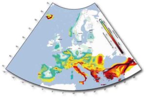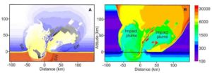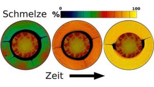

Simulation parameters for the scenario that generated the least shaking in the Seattle area. Credit: Erin Wirth/University of Washington/USGS
One of the worst nightmares for many Pacific Northwest residents is a huge earthquake along the offshore Cascadia Subduction Zone, which would unleash damaging and likely deadly shaking in coastal Washington, Oregon, British Columbia and northern California.
The last time this happened was in 1700, before seismic instruments were around to record the event. So what will happen when it ruptures next is largely unknown.
A University of Washington research project, to be presented Oct. 24 at the Geological Society of America’s annual meeting in Seattle, simulates 50 different ways that a magnitude-9.0 earthquake on the Cascadia subduction zone could unfold.
“There had been just a handful of detailed simulations of a magnitude-9 Cascadia earthquake, and it was hard to know if they were showing the full range,” said Erin Wirth, who led the project as a UW postdoctoral researcher in Earth and space sciences. “With just a few simulations you didn’t know if you were seeing a best-case, a worst-case or an average scenario. This project has really allowed us to be more confident in saying that we’re seeing the full range of possibilities.”
Off the Oregon and Washington coast, the Juan de Fuca oceanic plate is slowly moving under the North American plate. Geological clues show that it last jolted and unleashed a major earthquake in 1700, and that it does so roughly once every 500 years. It could happen any day.
Wirth’s project ran simulations using different combinations for three key factors: the epicenter of the earthquake; how far inland the earthquake will rupture; and which sections of the fault will generate the strongest shaking.
Results show that the intensity of shaking can be less for Seattle if the epicenter is fairly close to beneath the city. From that starting point, seismic waves will radiate away from Seattle, sending the biggest shakes in the direction of travel of the rupture.
“Surprisingly, Seattle experiences less severe shaking if the epicenter is located just beneath the tip of northwest Washington,” Wirth said. “The reason is because the rupture is propagating away from Seattle, so it’s most affecting sites offshore. But when the epicenter is located pretty far offshore, the rupture travels inland and all of that strong ground shaking piles up on its way to Seattle, to make the shaking in Seattle much stronger.”
The research effort began by establishing which factors most influence the pattern of ground shaking during a Cascadia earthquake. One, of course, is the epicenter, or more specifically the “hypocenter,” which locates the earthquake’s starting point in three-dimensional space.
Another factor they found to be important is how far inland the fault slips. A magnitude-9.0 earthquake would likely give way along the whole north-south extent of the subduction zone, but it’s not well known how far east the shake-producing area would extend, approaching the area beneath major cities such as Seattle and Portland.
The third factor is a new idea relating to a subduction zone’s stickiness. Earthquake researchers have become aware of the importance of “sticky points,” or areas between the plates that can catch and generate more shaking. This is still an area of current research, but comparisons of different seismic stations during the 2010 Chile earthquake and the 2011 Tohoku earthquake show that some parts of the fault released more strong shaking than others.
Wirth simulated a magnitude-9.0 earthquake, about the middle of the range of estimates for the magnitude of the 1700 earthquake. Her 50 simulations used variables spanning realistic values for the depth of the slip, and had randomly placed hypocenters and sticky points. The high-resolution simulations were run on supercomputers at the Pacific Northwest National Laboratory and the University of Texas, Austin.
Overall, the results confirm that coastal areas would be hardest hit, and locations in sediment-filled basins like downtown Seattle would shake more than hard, rocky mountaintops. But within that general framework, the picture can vary a lot; depending on the scenario, the intensity of shaking can vary by a factor of 10. But none of the pictures is rosy.
“We are finding large amplification of ground shaking by the Seattle basin,” said collaborator Art Frankel, a U.S. Geological Survey seismologist and affiliate faculty member at the UW. “The average duration of strong shaking in Seattle is about 100 seconds, about four times as long as from the 2001 Nisqually earthquake.”
The research was done as part of the M9 Project, a National Science Foundation-funded effort to figure out what a magnitude-9 earthquake might look like in the Pacific Northwest and how people can prepare. Two publications are being reviewed by the USGS, and engineers are already using the simulation results to assess how tall buildings in Seattle might respond to the predicted pattern of shaking.
As a new employee of the USGS, Wirth will now use geological clues to narrow down the possible earthquake scenarios.
“We’ve identified what parameters we think are important,” Wirth said. “I think there’s a future in using geologic evidence to constrain these parameters, and maybe improve our estimate of seismic hazard in the Pacific Northwest.”
An earthquake is the shaking of the surface of the Earth, resulting from the sudden release of energy in the Earth’s lithosphere that creates seismic waves. Earthquakes can range in size from those that are so weak that they cannot be felt to those violent enough to toss people around and destroy whole cities. The seismicity or seismic activity of an area refers to the frequency, type and size of earthquakes experienced over a period of time.
At the Earth’s surface, earthquakes manifest themselves by shaking and sometimes displacement of the ground. When the epicenter of a large earthquake is located offshore, the seabed may be displaced sufficiently to cause a tsunami. Earthquakes can also trigger landslides, and occasionally volcanic activity.
In its most general sense, the word earthquake is used to describe any seismic event — whether natural or caused by humans — that generates seismic waves. Earthquakes are caused mostly by rupture of geological faults, but also by other events such as volcanic activity, landslides, mine blasts, and nuclear tests. An earthquake’s point of initial rupture is called its focus or hypocenter. The epicenter is the point at ground level directly above the hypocenter.
What causes earthquakes and where do they happen?
The earth has four major layers: the inner core, outer core, mantle and crust. The crust and the top of the mantle make up a thin skin on the surface of our planet. But this skin is not all in one piece – it is made up of many pieces like a puzzle covering the surface of the earth. Not only that, but these puzzle pieces keep slowly moving around, sliding past one another and bumping into each other. We call these puzzle pieces tectonic plates, and the edges of the plates are called the plate boundaries. The plate boundaries are made up of many faults, and most of the earthquakes around the world occur on these faults. Since the edges of the plates are rough, they get stuck while the rest of the plate keeps moving. Finally, when the plate has moved far enough, the edges unstick on one of the faults and there is an earthquake.
Why does the earth shake when there is an earthquake?
While the edges of faults are stuck together, and the rest of the block is moving, the energy that would normally cause the blocks to slide past one another is being stored up. When the force of the moving blocks finally overcomes the friction of the jagged edges of the fault and it unsticks, all that stored up energy is released. The energy radiates outward from the fault in all directions in the form of seismic waves like ripples on a pond. The seismic waves shake the earth as they move through it, and when the waves reach the earth’s surface, they shake the ground and anything on it, like our houses and us! (see P&S Wave inset)
How are earthquakes recorded?
Earthquakes are recorded by instruments called seismographs. The recording they make is called a seismogram. The seismograph has a base that sets firmly in the ground, and a heavy weight that hangs free. When an earthquake causes the ground to shake, the base of the seismograph shakes too, but the hanging weight does not. Instead the spring or string that it is hanging from absorbs all the movement. The difference in position between the shaking part of the seismograph and the motionless part is what is recorded.
How do scientists measure the size of earthquakes?
The size of an earthquake depends on the size of the fault and the amount of slip on the fault, but that’s not something scientists can simply measure with a measuring tape since faults are many kilometers deep beneath the earth’s surface. So how do they measure an earthquake? They use the seismogram recordings made on the seismographs at the surface of the earth to determine how large the earthquake was. A short wiggly line that doesn’t wiggle very much means a small earthquake, and a long wiggly line that wiggles a lot means a large earthquake. The length of the wiggle depends on the size of the fault, and the size of the wiggle depends on the amount of slip.
The size of the earthquake is called its magnitude. There is one magnitude for each earthquake. Scientists also talk about the intensity of shaking from an earthquake, and this varies depending on where you are during the earthquake.
How can scientists tell where the earthquake happened?
Seismograms come in handy for locating earthquakes too, and being able to see the P wave and the S wave is important. You learned how P & S waves each shake the ground in different ways as they travel through it. P waves are also faster than S waves, and this fact is what allows us to tell where an earthquake was. To understand how this works, let’s compare P and S waves to lightning and thunder. Light travels faster than sound, so during a thunderstorm you will first see the lightning and then you will hear the thunder. If you are close to the lightning, the thunder will boom right after the lightning, but if you are far away from the lightning, you can count several seconds before you hear the thunder. The further you are from the storm, the longer it will take between the lightning and the thunder.
P waves are like the lightning, and S waves are like the thunder. The P waves travel faster and shake the ground where you are first. Then the S waves follow and shake the ground also. If you are close to the earthquake, the P and S wave will come one right after the other, but if you are far away, there will be more time between the two. By looking at the amount of time between the P and S wave on a seismogram recorded on a seismograph, scientists can tell how far away the earthquake was from that location. However, they can’t tell in what direction from the seismograph the earthquake was, only how far away it was. If they draw a circle on a map around the station where the radius of the circle is the determined distance to the earthquake, they know the earthquake lies somewhere on the circle. But where?
Scientists then use a method called triangulation to determine exactly where the earthquake was (figure 6). It is called triangulation because a triangle has three sides, and it takes three seismographs to locate an earthquake. If you draw a circle on a map around three different seismographs where the radius of each is the distance from that station to the earthquake, the intersection of those three circles is the epicenter!
Can scientists predict earthquakes?
No, and it is unlikely they will ever be able to predict them. Scientists have tried many different ways of predicting earthquakes, but none have been successful. On any particular fault, scientists know there will be another earthquake sometime in the future, but they have no way of telling when it will happen.
Effects of earthquakes
Shaking and ground rupture
Shaking and ground rupture are the main effects created by earthquakes, principally resulting in more or less severe damage to buildings and other rigid structures. The severity of the local effects depends on the complex combination of the earthquake magnitude, the distance from the epicenter, and the local geological and geomorphological conditions, which may amplify or reduce wave propagation. The ground-shaking is measured by ground acceleration.
Specific local geological, geomorphological, and geostructural features can induce high levels of shaking on the ground surface even from low-intensity earthquakes. This effect is called site or local amplification. It is principally due to the transfer of the seismic motion from hard deep soils to soft superficial soils and to effects of seismic energy focalization owing to typical geometrical setting of the deposits.
Ground rupture is a visible breaking and displacement of the Earth’s surface along the trace of the fault, which may be of the order of several meters in the case of major earthquakes. Ground rupture is a major risk for large engineering structures such as dams, bridges and nuclear power stations and requires careful mapping of existing faults to identify any which are likely to break the ground surface within the life of the structure.
Landslides and avalanches
Earthquakes, along with severe storms, volcanic activity, coastal wave attack, and wildfires, can produce slope instability leading to landslides, a major geological hazard. Landslide danger may persist while emergency personnel are attempting rescue.
Fires
Earthquakes can cause fires by damaging electrical power or gas lines. In the event of water mains rupturing and a loss of pressure, it may also become difficult to stop the spread of a fire once it has started. For example, more deaths in the 1906 San Francisco earthquake were caused by fire than by the earthquake itself.
Soil liquefaction
Soil liquefaction occurs when, because of the shaking, water-saturated granular material (such as sand) temporarily loses its strength and transforms from a solid to a liquid. Soil liquefaction may cause rigid structures, like buildings and bridges, to tilt or sink into the liquefied deposits. For example, in the 1964 Alaska earthquake, soil liquefaction caused many buildings to sink into the ground, eventually collapsing upon themselves.
Tsunami
Tsunamis are long-wavelength, long-period sea waves produced by the sudden or abrupt movement of large volumes of water – including when an earthquake occurs at sea. In the open ocean the distance between wave crests can surpass 100 kilometers (62 mi), and the wave periods can vary from five minutes to one hour. Such tsunamis travel 600-800 kilometers per hour (373–497 miles per hour), depending on water depth. Large waves produced by an earthquake or a submarine landslide can overrun nearby coastal areas in a matter of minutes. Tsunamis can also travel thousands of kilometers across open ocean and wreak destruction on far shores hours after the earthquake that generated them.
Ordinarily, subduction earthquakes under magnitude 7.5 on the Richter magnitude scale do not cause tsunamis, although some instances of this have been recorded. Most destructive tsunamis are caused by earthquakes of magnitude 7.5 or more. “ex: Japan Tsunami 2011”
Floods
A flood is an overflow of any amount of water that reaches land. Floods occur usually when the volume of water within a body of water, such as a river or lake, exceeds the total capacity of the formation, and as a result some of the water flows or sits outside of the normal perimeter of the body. However, floods may be secondary effects of earthquakes, if dams are damaged. Earthquakes may cause landslips to dam rivers, which collapse and cause floods.
The terrain below the Sarez Lake in Tajikistan is in danger of catastrophic flood if the landslide dam formed by the earthquake, known as the Usoi Dam, were to fail during a future earthquake. Impact projections suggest the flood could affect roughly 5 million people.
Haiti Earthquake. Credit: United Nations Development Programme
A group of researchers from the UK and the US have used machine learning techniques to successfully predict earthquakes. Although their work was performed in a laboratory setting, the experiment closely mimics real-life conditions, and the results could be used to predict the timing of a real earthquake.
The team, from the University of Cambridge, Los Alamos National Laboratory and Boston University, identified a hidden signal leading up to earthquakes, and used this ‘fingerprint’ to train a machine learning algorithm to predict future earthquakes. Their results, which could also be applied to avalanches, landslides and more, are reported in the journal Geophysical Review Letters.
For geoscientists, predicting the timing and magnitude of an earthquake is a fundamental goal. Generally speaking, pinpointing where an earthquake will occur is fairly straightforward: if an earthquake has struck a particular place before, the chances are it will strike there again. The questions that have challenged scientists for decades are how to pinpoint when an earthquake will occur, and how severe it will be. Over the past 15 years, advances in instrument precision have been made, but a reliable earthquake prediction technique has not yet been developed.
As part of a project searching for ways to use machine learning techniques to make gallium nitride (GaN) LEDs more efficient, the study’s first author, Bertrand Rouet-Leduc, who was then a PhD student at Cambridge, moved to Los Alamos National Laboratory in New Mexico to start a collaboration on machine learning in materials science between Cambridge University and Los Alamos. From there the team started helping the Los Alamos Geophysics group on machine learning questions.
The team at Los Alamos, led by Paul Johnson, studies the interactions among earthquakes, precursor quakes (often very small earth movements) and faults, with the hope of developing a method to predict earthquakes. Using a lab-based system that mimics real earthquakes, the researchers used machine learning techniques to analyse the acoustic signals coming from the ‘fault’ as it moved and search for patterns.
The laboratory apparatus uses steel blocks to closely mimic the physical forces at work in a real earthquake, and also records the seismic signals and sounds that are emitted. Machine learning is then used to find the relationship between the acoustic signal coming from the fault and how close it is to failing.
The machine learning algorithm was able to identify a particular pattern in the sound, previously thought to be nothing more than noise, which occurs long before an earthquake. The characteristics of this sound pattern can be used to give a precise estimate (within a few percent) of the stress on the fault (that is, how much force is it under) and to estimate the time remaining before failure, which gets more and more precise as failure approaches. The team now thinks that this sound pattern is a direct measure of the elastic energy that is in the system at a given time.
“This is the first time that machine learning has been used to analyse acoustic data to predict when an earthquake will occur, long before it does, so that plenty of warning time can be given – it’s incredible what machine learning can do,” said co-author Professor Sir Colin Humphreys of Cambridge’s Department of Materials Science & Metallurgy, whose main area of research is energy-efficient and cost-effective LEDs. Humphreys was Rouet-Leduc’s supervisor when he was a PhD student at Cambridge.
“Machine learning enables the analysis of datasets too large to handle manually and looks at data in an unbiased way that enables discoveries to be made,” said Rouet-Leduc.
Although the researchers caution that there are multiple differences between a lab-based experiment and a real earthquake, they hope to progressively scale up their approach by applying it to real systems which most resemble their lab system. One such site is in California along the San Andreas Fault, where characteristic small repeating earthquakes are similar to those in the lab-based earthquake simulator. Progress is also being made on the Cascadia fault in the Pacific Northwest of the United States and British Columbia, Canada, where repeating slow earthquakes that occur over weeks or months are also very similar to laboratory earthquakes.
“We’re at a point where huge advances in instrumentation, machine learning, faster computers and our ability to handle massive data sets could bring about huge advances in earthquake science,” said Rouet-Leduc.
Reference:
Bertrand Rouet-Leduc et al, Machine Learning Predicts Laboratory Earthquakes, Geophysical Research Letters (2017). DOI: 10.1002/2017GL074677
Lithospheric-scale processes involved in the precursor stage of formation of the Deseado Massif auriferous province. Stage A: plume activity during Early Jurassic related to the initial stages of Gondwana break-up induces metasomatic Au enrichment in the overlying SCLM and coeval partial melting. The inset shows the transfer of Au to the enriched domains and partial melting processes responsible for the early magmatic stages of the CA-SLIP. Stage B: onset of the subduction zone at the western margin of Gondwana provides fluids capable of scavenging Au from formerly enriched domains and generates calc-alkaline magmatism represented by the middle-late magmatic stages of the CA-SLIP that hosts the Au deposits. The inset shows the process of partial melting of enriched domains and Au transport to crustal levels; some portions of enriched lithosphere remain unmodified
Gold enrichment at the crustal or mantle source has been proposed as a key ingredient in the production of giant gold deposits and districts. However, the lithospheric-scale processes controlling gold endowment in a given metallogenic province remain unclear.
Here we provide the first direct evidence of native gold in the mantle beneath the Deseado Massif in Patagonia that links an enriched mantle source to the occurrence of a large auriferous province in the overlying crust. A precursor stage of mantle refertilisation by plume-derived melts generated a gold-rich mantle source during the Early Jurassic.
The interplay of this enriched mantle domain and subduction-related fluids released during the Middle-Late Jurassic resulted in optimal conditions to produce the ore-forming magmas that generated the gold deposits. Our study highlights that refertilisation of the subcontinental lithospheric mantle is a key factor in forming large metallogenic provinces in the Earth’s crust, thus providing an alternative view to current crust-related enrichment models.
The traditional notion of Au endowment in a given metallogenic province is that Au accumulates by highly efficient magmatic-hydrothermal enrichment processes operating in a chemically ‘average’ crust. However, more recent views point to anomalously enriched source regions and/or melts that are critical for the formation of Au provinces at a lithospheric scale. Within this perspective, Au-rich melts/fluids might originate from a mid or lower crust reservoir and later migrate through favourable structural zones to shallower crustal levels where the Au deposits form. Alternatively, the subcontinental lithospheric mantle (SCLM) may also play a role as a source of metal-rich magmas.
This model involves deep-seated Au-rich magmas that may infiltrate the edges of buoyant and rigid domains in the SCLM producing transient Au storage zones. Upon melting, the ascending magma scavenges the Au as it migrates towards the uppermost overlying crust. Discontinuities between buoyant and rigid domains in the SCLM provide the channelways for the uprising of Au-rich fluids or melts from the convecting underlying mantle, and when connected to the overlying crust by trans-lithospheric faults, a large Au deposit or well-endowed auriferous province can be formed. Thus, the generation of Au deposits in the crust may result from the conjunction in time and space of three essential factors: an upper mantle or lower crustal source region particularly enriched in Au, a transient remobilisation event and favourable lithospheric-scale plumbing structures.
The giant Ladolam Au deposit in Papua New Guinea gives a good single-deposit case example of this mechanism since deep trans-lithospheric faults connect the crustal Au deposit directly with the mantle source, and similar Os isotopic compositions are exhibited by Au ores and metal-enriched peridotite of the underlying mantle. Despite these evidences, the genetic relation between a pre-enriched mantle source and the occurrence of gold provinces in the upper crust remains controversial since limited evidence is available at a broader regional scale.
The layer of the Earth we live on is broken into a dozen or so rigid slabs (called tectonic plates by geologists) that are moving relative to one another. Credit: USGS
Plate tectonics is a scientific theory describing the large-scale motion of seven large plates and the movements of a larger number of smaller plates of the Earth’s lithosphere, since tectonic processes began on Earth between 3 and 3.5 billion years ago. The model builds on the concept of continental drift, an idea developed during the first decades of the 20th century. The geoscientific community accepted plate-tectonic theory after seafloor spreading was validated in the late 1950s and early 1960s.
The lithosphere, which is the rigid outermost shell of a planet (the crust and upper mantle), is broken into tectonic plates. The Earth’s lithosphere is composed of seven or eight major plates (depending on how they are defined) and many minor plates. Where the plates meet, their relative motion determines the type of boundary: convergent, divergent, or transform. Earthquakes, volcanic activity, mountain-building, and oceanic trench formation occur along these plate boundaries (or faults). The relative movement of the plates typically ranges from zero to 100 mm annually.
How do these massive slabs of solid rock float despite their tremendous weight?
The answer lies in the composition of the rocks. Continental crust is composed of granitic rocks which are made up of relatively lightweight minerals such as quartz and feldspar. By contrast, oceanic crust is composed of basaltic rocks, which are much denser and heavier. The variations in plate thickness are nature’s way of partly compensating for the imbalance in the weight and density of the two types of crust. Because continental rocks are much lighter, the crust under the continents is much thicker (as much as 100 km) whereas the crust under the oceans is generally only about 5 km thick. Like icebergs, only the tips of which are visible above water, continents have deep “roots” to support their elevations.
How did oceanic plate boundaries mapped?
Most of the boundaries between individual plates cannot be seen, because they are hidden beneath the oceans. Yet oceanic plate boundaries can be mapped accurately from outer space by measurements from GEOSAT satellites. Earthquake and volcanic activity is concentrated near these boundaries. Tectonic plates probably developed very early in the Earth’s 4.6-billion-year history, and they have been drifting about on the surface ever since-like slow-moving bumper cars repeatedly clustering together and then separating.
Types of plate boundaries
Transform boundaries
Transform boundaries (Conservative) occur where two lithospheric plates slide, or perhaps more accurately, grind past each other along transform faults, where plates are neither created nor destroyed. The relative motion of the two plates is either sinistral (left side toward the observer) or dextral (right side toward the observer). Transform faults occur across a spreading center. Strong earthquakes can occur along a fault. The San Andreas Fault in California is an example of a transform boundary exhibiting dextral motion.
Divergent boundaries
Divergent boundaries (Constructive) occur where two plates slide apart from each other. At zones of ocean-to-ocean rifting, divergent boundaries form by seafloor spreading, allowing for the formation of new ocean basin. As the ocean plate splits, the ridge forms at the spreading center, the ocean basin expands, and finally, the plate area increases causing many small volcanoes and/or shallow earthquakes. At zones of continent-to-continent rifting, divergent boundaries may cause new ocean basin to form as the continent splits, spreads, the central rift collapses, and ocean fills the basin. Active zones of Mid-ocean ridges (e.g., Mid-Atlantic Ridge and East Pacific Rise), and continent-to-continent rifting (such as Africa’s East African Rift and Valley, Red Sea) are examples of divergent boundaries.
Convergent boundaries
Convergent boundary, also known as a destructive plate boundary, is a region of active deformation where two or more tectonic plates or fragments of the lithosphere near the end of their life cycle. This is in contrast to a constructive plate boundary (also known as a mid-ocean ridge or spreading center). As a result of pressure, friction, and plate material melting in the mantle, earthquakes and volcanoes are common near destructive boundaries, where subduction zones or an area of continental collision (depending on the nature of the plates involved) occurs. The subducting plate in a subduction zone is normally oceanic crust, and moves beneath the other plate, which can be made of either oceanic or continental crust. During collisions between two continental plates, large mountain ranges, such as the Himalayas are formed. In other regions, a divergent boundary or transform faults may be present.
Toe bones, the upper jaw and snout of the fossilized remains of a tyrannosaur skeleton found in Grand Staircase-Escalante National Monument. The skeleton is the most complete of its kind found in the Southwest United States. Credit: Mark Johnston/NHMU
A remarkable new fossilized skeleton of a tyrannosaur discovered in the Bureau of Land Management’s Grand Staircase-Escalante National Monument (GSENM) in southern Utah was airlifted by helicopter Sunday, Oct 15, from a remote field site, and delivered to the Natural History Museum of Utah where it will be uncovered, prepared, and studied. The fossil is approximately 76 million years old and is most likely an individual of the species Teratophoneus curriei, one of Utah’s ferocious tyrannosaurs that walked western North America between 66 and 90 million years ago during the Late Cretaceous Period.
“With at least 75 percent of its bones preserved, this is the most complete skeleton of a tyrannosaur ever discovered in the southwestern US,” said Dr. Randall Irmis, curator of paleontology at the Museum and associate professor in the Department of Geology and Geophysics at the University of Utah. “We are eager to get a closer look at this fossil to learn more about the southern tyrannosaur’s anatomy, biology, and evolution.”
GSENM Paleontologist Dr. Alan Titus discovered the fossil in July 2015 in the Kaiparowits Formation, part of the central plateau region of the monument. Particularly notable is that the fossil includes a nearly complete skull. Scientists hypothesize that this tyrannosaur was buried either in a river channel or by a flooding event on the floodplain, keeping the skeleton intact.
“The monument is a complex mix of topography — from high desert to badlands — and most of the surface area is exposed rock, making it rich grounds for new discoveries, said Titus. “And we’re not just finding dinosaurs, but also crocodiles, turtles, mammals, amphibians, fish, invertebrates, and plant fossils — remains of a unique ecosystem not found anywhere else in the world,” said Titus.
Although many tyrannosaur fossils have been found over the last one hundred years in the northern Great Plains region of the northern US and Canada, until relatively recently, little was known about them in the southern US. This discovery, and the resulting research, will continue to cement the monument as a key place for understanding the group’s southern history, which appears to have followed a different path than that of their northern counterparts.
This southern tyrannosaur fossil is thought to be a sub-adult individual, 12-15 years old, 17-20 feet long, and with a relatively short head, unlike the typically longer-snouted look of northern tyrannosaurs.
Collecting such fossils from the monument can be unusually challenging. “Many areas are so remote that often we need to have supplies dropped in and the crew hikes in,” said Irmis. For this particular field site, Museum and monument crews back-packed in, carrying all of the supplies they needed to excavate the fossil, such as plaster, water and tools to work at the site for several weeks. The crews conducted a three-week excavation in early May 2017, and continued work during the past two weeks until the specimen was ready to be airlifted out.
Irmis said with the help of dedicated volunteers, it took approximately 2,000-3,000 people hours to excavate the site and estimates at least 10,000 hours of work remain to prepare the specimen for research. “Without our volunteer team members, we wouldn’t be able to accomplish this work. We absolutely rely on them throughout the entire process,” said Irmis.
Irmis says that this new fossil find is extremely significant. Whether it is a new species or an individual of Teratophoneus, the new research will provide important context as to how this animal lived. “We’ll look at the size of this new fossil, it’s growth pattern, biology, reconstruct muscles to see how the animal moved, how fast could it run, and how it fed with its jaws. The possibilities are endless and exciting,” said Irmis.
During the past 20 years, crews from the Natural History Museum of Utah and GSENM have unearthed more than a dozen new species of dinosaurs in GSENM, with several additional species awaiting formal scientific description. Some of the finds include another tyrannosaur named Lythronax, and a variety of other plant-eating dinosaurs — among them duck-billed hadrosaurs, armored ankylosaurs, dome-headed pachycephalosaurs, and a number of horned dinosaurs, such as Utahceratops, Kosmoceratops, Nasutoceratops, and Machairoceratops. Other fossil discoveries include fossil plants, insect traces, snails, clams, fishes, amphibians, lizards, turtles, crocodiles, and mammals. Together, this diverse bounty of fossils is offering one of the most comprehensive glimpses into a Mesozoic ecosystem. Remarkably, virtually all of the dinosaur species found in GSENM appear to be unique to this area, and are not found anywhere else on Earth
An international expedition aims to better understand seismic activity through samples collected from one of the most geologically active areas in Europe.
More than 30 scientists, including Dr Richard Collier from the University of Leeds, will be participating in an expedition which will analyse data gathered from a tear in the ocean floor – the Corinth Rift.
The rift is caused by one of the Earth’s tectonic plates being ripped apart causing such geological hazards as earthquakes.
The overall aim of the project is to gain insight into the rifting process by collecting sediment cores and compiling data from the samples on their geological history, composition, age and structure.
The research vessel, DV Fugro Synergy, will launch in late October to collect the cores at three different locations with drilling going to a depth of 750 metres below the seabed.
Dr Collier, from the School of Earth and Environment at Leeds said: “The Corinth Rift provides a unique laboratory in one of the most seismically active areas in Europe. It is a relatively young tectonic feature having only formed in the last five million years. It is an ideal location to learn more about early rift development and how tectonics affect the landscape.
“The cores will also allow us to determine the relative impacts of sea level change of and climate change through time on the transfer of sediment from the surrounding landscape to the basin floor.
“The opportunity to quantify these competing controls on rift sedimentation for the first time makes this project particularly exciting. By increasing our understanding of this particular rift we may be better able to predict seismic hazards in other areas and inform the hunt for sediment bodies in other parts of the world that might contain hydrocarbons. ”
Researchers have been working in the Gulf of Corinth region for many decades – examining sediments and active fault traces exposed on land and using marine geophysics to image the basin and its structure below the seafloor. But there is very little information about the age of the sediments and of the environment of the rift in the last one to two million years.
The core samples collected and analysed by the team will help answer such questions as: What are the implications for earthquake activity in a developing rift? How does the rift actually evolve and grow and on what timescale? How did the activity on faults change with time? How does the landscape respond to tectonic and climatic changes? And what was the climate and the environment of the rift basin in the last one to two million years?
Co-chief scientist of the expedition, Professor Lisa McNeill from the University of Southampton, said: “By drilling, we hope to find this last piece of the jigsaw puzzle. It will help us to unravel the sequence of events as the rift has evolved and, importantly, how fast the faults, which regularly generate damaging earthquakes, are slipping.”
The 33 scientists involved in the expedition are from Australia, Brazil, China, France, Germany, Greece, India, Norway, Spain, the United States, and the United Kingdom and cover a range of different geoscience disciplines.
Nine of them will sail onboard the drill ship Fugro Synergy from October to December of this year. After the offshore phase in the Gulf of Corinth the entire team, including Dr Collier, will meet for the first time at the IODP Bremen Core Repository (BCR), located at MARUM – Center for Marine Environmental Sciences at the University of Bremen, Germany. There they will spend a month splitting, analysing and sampling the cores and reviewing the data collected.
Seismogram being recorded by a seismograph at the Weston Observatory in Massachusetts, USA. Credit: Wikipedia
A new database showcasing hundreds of examples of human-triggered earthquakes should shake up policy-makers, regulators and industry executives looking to mitigate these unacceptable hazards caused by our own actions, according to a Western Earth Sciences professor.
“More and more, we are recognizing how many earthquakes are actually human-induced,” said Gail Atkinson, Industrial Research Chair in Hazards from Induced Seismicity at Western.
“Researchers at the U.S. Geological Survey are now raising the possibility many of the large, well-known earthquakes in California that happened over the 1930s-50s – like the Long Beach Earthquake (in 1933) or the Kern County Earthquake (in 1952), which was a magnitude of 7.5 – may have been induced by oil-production in southern California at the time,” she explained.
Atkinson’s research group is studying this phenomenon of human-triggered earthquakes – or, induced seismicity – in western Canada, with a particular focus in Alberta. Her team has found evidence showing a significant increase in the number of earthquakes in the last five years or so in the active region. More than half of those appear to be related to hydraulic fracturing.
These findings are included in the new Human-Induced Earthquake Database – or HiQuake – which contains 728 examples of earthquakes (or sequences of earthquakes) that may have been set off by humans over the past 149 years.
While her team has uncovered evidence linking hydraulic fracturing to an increase in earthquakes, research also suggests a link between earthquakes and wastewater disposal in Alberta.
“There’s only a relatively small fraction of earthquakes purely tectonic or natural – so most of the seismicity we see in western Alberta and eastern British Columbia appears to be related to the oil and gas industry,” Atkinson noted.
“And that’s been raising a whole host of new issues in terms of how we should be planning and regulating hydraulic fracturing and oil and gas activity so we’re not causing unacceptable hazards – from seismic activity in particular – and ensuring we don’t conduct fracturing operations close to major infrastructure such as major dams or cortical facilities that (we don’t want to damage).”
With all these findings of human-induced seismicity emerging, and a new encyclopedic database storing the instances, researchers have been trying to wedge themselves between science and public policy in order to mitigate damage caused by human-triggered earthquakes, she continued.
“We’ve been trying to translate that knowledge into suggested guidelines, for example, for exclusion zones around critical infrastructures. We’ve suggested there shouldn’t be any hydraulic fracturing within 5 km of major dams or critical infrastructure,” Atkinson said.
“That’s the beginning. We’re working with regulators and policy-makers to try to get those ideas out there. The ideas are gaining traction. With some of the larger players – oil companies, Canadian associations for petroleum producers, and so on – if we can get them to start building that kind of thinking into best practices, that might actually be more achievable than regulation, which seems difficult to enforce. We’ve certainly started a dialogue; we have people talking. But how to translate findings into concrete policy, that is going to take time.”
Having something like HiQuake compile all documented instances of human-triggered earthquakes in one place makes it easier for researchers when they try to conduct studies establishing links between factors, Atkinson continued, adding this establishes the possibility of, at the very least, mitigating damage caused by such events.
“Unlike with natural earthquake hazards, we can do something about this. That’s what really motivates us. Whereas, with natural hazards, you can’t do anything about it, other than be prepared. You can’t stop an earthquake from happening; you can’t predict where it might happen. Similarly, with other natural disasters like hurricanes, you can be prepared, but you can’t stop it.
“This is something within our power to control. We really do have an opportunity here to make sure we don’t cause a major environmental disaster through actions we’ve taken that we didn’t need to take.”
New Macquarie University research, published in the journal Proceedings of the Royal Society B, has shown that birds and pterosaurs did, in fact, co-exist for millions of years peacefully, as opposed to the long-held and historical belief that birds competitively-displaced pterosaurs as suggested.
It had previously been suggested that birds and pterosaurs competed with each other during the Cretaceous, a period more than 65 million years ago, and that this led to pterosaurs evolving larger body sizes to avoid competition with the smaller birds. However, after comparing jaw sizes, limb proportions and other functional characteristics not explored in previous studies, lead author Dr Nicholas Chan says this is not the case.
The research used morphospaces, a way of mapping the forms of organisms, and found distinct ecological separation between the two groups based on size, features of the wings and legs and feeding adaptations. In other words, this would suggest that the two were not long term competitors. Had the two been in direct competition, birds were believed to have been the reason that pterosaurs evolved into larger species in order to avoid competition for resources.
“Any competition between the two groups was likely localised over a relatively short periods of time,” says Dr Chan, from the Department of Biological Sciences at Macquarie University.
“While previous research only compared the limb bones of the two groups, our research compared jaw lengths, wing and leg proportions in order to determine functionally-equivalent traits, and found that the there was very little ecomophological overlap between the two.”
“The difference in the species functional morphology means that both groups co-existed without ongoing competition. Birds had shorter mid-wings, longer metatarsals, and shorter jaws. So they likely flew, walked, and fed differently from pterosaurs.”
Reference:
Nicholas R. Chan. Morphospaces of functionally analogous traits show ecological separation between birds and pterosaurs, Proceedings of the Royal Society B: Biological Sciences (2017). DOI: 10.1098/rspb.2017.1556
This map shows the elevation change of Mount Rainier glaciers between 1970 and 2016. The earlier observations are from USGS maps, while the recent data use the satellite stereo imaging technique. Glacier surface elevations have dropped more than 40 meters (130 feet) in some places. Credit: David Shean/University of Washington
Until recently, glaciers in the United States have been measured in two ways: placing stakes in the snow, as federal scientists have done each year since 1957 at South Cascade Glacier in Washington state; or tracking glacier area using photographs from airplanes and satellites.
We now have a third, much more powerful tool. While he was a doctoral student in University of Washington’s Department of Earth and Space Sciences, David Shean devised new ways to use high-resolution satellite images to track elevation changes for massive ice sheets in Antarctica and Greenland. Over the years he wondered: Why aren’t we doing this for mountain glaciers in the United States, like the one visible from his department’s office window?
He has now made that a reality. In 2012, he first asked for satellite time to turn digital eyes on glaciers in the continental U.S., and he has since collected enough data to analyze mass loss for Mount Rainier and almost all the glaciers in the lower 48 states. He will present results from these efforts Oct. 22 at the Geological Society of America’s annual meeting in Seattle.
“I’m interested in the broad picture: What is the state of all of the glaciers, and how has that changed over the last 50 years? How has that changed over the last 10 years? And at this point, how are they changing every year?” said Shean, who is now a research associate with the UW’s Applied Physics Laboratory.
The maps provide a twice-yearly tally of roughly 1,200 mountain glaciers in the lower 48 states, down to a resolution of about 1 foot. Most of those glaciers are in Washington state, with others clustered in the Rocky Mountains of Montana, Wyoming and Colorado, and in California’s Sierra Nevada.
To create the maps, a satellite camera roughly half the size of the Hubble Space Telescope must take two images of a glacier from slightly different angles. As the satellite passes overhead, moving at about 4.6 miles per second, it takes images a few minutes apart. Each pixel of the image covers 30 to 50 centimeters (about 1 foot) and a single image can be tens of miles across.
Shean’s technique uses automated software that matches millions of small features, such as rocks or crevasses, in the two images. It then uses the difference in perspective to create a 3-D model of the surface.
The first such map of a Mount St. Helens glacier was obtained in 2012, and the first for Mount Rainier in 2014. The project has grown steadily since then to include more glaciers every year.
The results confirm stake measurements at South Cascade Glacier, showing significant loss over the past 60 years. Results at Mount Rainier also reflect the broader shrinking trends, with the lower-elevation glaciers being particularly hard hit. Shean estimates cumulative ice loss of about 0.7 cubic kilometers (900 million cubic yards) at Mount Rainier since 1970. Distributed evenly across all of Mount Rainier’s glaciers, that’s equivalent to removing a layer of ice about 25 feet (7 to 8 meters) thick.
“There are some big changes that have happened, as anyone who’s been hiking on Mount Rainier in the last 45 years can attest to,” Shean said. “For the first time we’re able to very precisely quantify exactly how much snow and ice has been lost.”
The glacier loss at Rainier is consistent with trends for glaciers across the U.S. and worldwide. Tracking the status of so many glaciers will allow scientists to further explore patterns in the changes over time, which will help pinpoint the causes — from changes in temperature and precipitation to slope angle and elevation.
“The next step is to integrate our observations with glacier and climate models and say: Based on what we know now, where are these systems headed?” Shean said.
Those predictions could be used to better manage water supplies and flood risks.
“We want to know what the glaciers are doing and how their mass is changing, but it’s important to remember that the meltwater is going somewhere. It ends up in rivers, it ends up in reservoirs, it ends up downstream in the ocean. So there are very real applications for water resource management,” Shean said. “If we know how much snow falls on Mount Rainier every winter, and when and how much ice melts every summer, that can inform water resource managers’ decisions.”
Davidsmithite, a newly approved feldspathoid mineral (IMA 2016-070), occurs as a rock-forming mineral in the Liset eclogite pod (Norwegian Caledonides).
The approved electron-microprobe analysis gave the crystal–chemical formula: ([Ca0.636◰0.636]◰0.414K0.165Na0.149)Σ2.000Na6.000(Al7.863Fe3+0.019)Σ7.882Si8.192O32 (where ◰ = vacancy)
Davidsmithite completes the compositional space of the nepheline-structure group by providing a new root-composition, (Ca◰)2Na6Al8Si8O32. It is the Ca-analogue of classical nepheline, to which it is related by the heterovalent substitution of K+2 by [Ca2+◰]. Most of the Ca2+ ions are situated in the same atomic position as K+ in nepheline, but some occur in a new and disordered (Ca′) atomic position, whose centre is shifted by 2.18 Å along the 6-fold axis.
The studied samples show some solid-solution towards the other two possible end-members of the nepheline compositional space, so that the channel site contains all of Ca and K in the unit formula, with some Na and â—°. In the Liset eclogite pod, davidsmithite occurs in retrogressed, formerly jadeite-rich zones; it commonly overgrows lisetite and is associated with albitic plagioclase and taramitic amphibole.
This eclogite occurrence is noted for its bulk-rock compositions rich in (Na + Al) and poor in growth of a (K + Mg). The paucity in K prevented the growth of nepheline, and the paucity in Si in precursor jadeite led to the growth of a feldspathoid (davidsmithite) as well as of lisetite; a feldspar (albite or oligoclase) also occurs nearby.
Sid-Ali Kechid, Gian Carlo Parodi, Sylvain Pont, Roberta Oberti. Davidsmithite, (Ca,â—°)2Na6Al8Si8O32: a new, Ca-bearing nepheline-group mineral from the Western Gneiss Region, Norway. DOI: 10.1127/ejm/2017/0029-2667 Published on June 2017, First Published on June 28, 2017
Smith, D.C., Kechid, S-A. and Rossi, G. (1986): Occurence and properties of lisetite, CaNa2Al4Si4O16, a new tectosilicate in the system Ca-Na-Al-Si-O. American Mineralogist 71, 1372-1377. [as K-poor, Ca-rich nepheline structure mineral]
Kechid, S.-A., Oberti, R., Rossi, G., Parodi, G., Pont, P. (2016): Davidsmithite, IMA 2016-070. CNMNC Newsletter No. 34, December 2016, page 1317; Mineralogical Magazine: 80: 1315–1321
A turquoise artifact linked to Canyon Creek. Credit: Saul Hedquist
Turquoise is an icon of the desert Southwest, with enduring cultural significance, especially for Native American communities. Yet, relatively little is known about the early history of turquoise procurement and exchange in the region.
University of Arizona researchers are starting to change that by blending archaeology and geochemistry to get a more complete picture of the mineral’s mining and distribution in the region prior to the 16th-century arrival of the Spanish.
In a new paper, published in the November issue of the Journal of Archaeological Science, UA anthropology alumnus Saul Hedquist and his collaborators revisit what once was believed to be a relatively small turquoise mine in eastern Arizona. Their findings suggest that the Canyon Creek mine, located on the White Mountain Apache Indian Reservation, was actually a much more significant source of turquoise than previously thought.
With permission from the White Mountain Apache Tribe, Hedquist and his colleagues visited the now essentially exhausted Canyon Creek source—which has been known to archaeologists since the 1930s—to remap the area and collect new samples. There, they found evidence of previously undocumented mining areas, which suggest the output of the mine may have been 25 percent higher than past surveys indicated.
“Pre-Hispanic workings at Canyon Creek were much larger than previously estimated, so the mine was clearly an important source of turquoise while it was active,” said Hedquist, lead author of the paper, who earned his doctorate from the UA School of Anthropology in the College of Social and Behavioral Sciences in May.
In addition, the researchers measured ratios of lead and strontium isotopes in samples they collected from the mine, and determined that Canyon Creek turquoise has a unique isotopic fingerprint that distinguishes it from other known turquoise sources in the Southwest. The isotopic analysis was conducted in the lab of UA College of Science Dean Joaquin Ruiz in the Department of Geosciences by study co-author and UA geosciences alumna Alyson Thibodeau. Now an assistant professor at Dickinson College in Pennsylvania, Thibodeau did her UA dissertation on isotopic fingerprinting of geological sources of turquoise throughout the Southwest.
“If you pick up a piece of turquoise from an archaeological site and say ‘where does it come from?’ you have to have some means of telling the different turquoise deposits apart,” said David Killick, UA professor of anthropology, who co-authored the paper with Hedquist, Thibodeau and John Welch, a UA alumnus now on the faculty at Simon Fraser University. “Alyson’s work shows that the major mining areas can be distinguished by measurement of major lead and strontium isotopic ratios.”
Based on the isotopic analysis, researchers were able to confidently match turquoise samples they collected at Canyon Creek to several archaeological artifacts housed in museums. Their samples matched artifacts that had been uncovered at sites throughout much of east-central Arizona—some more than 100 kilometers from the mine—suggesting that distribution of Canyon Creek turquoise was broader than previously thought, and that the mine was a significant source of turquoise for pre-Hispanic inhabitants of the Mogollon Rim area.
The researchers also were able to pinpoint when the mine was most active. Their samples matched artifacts found at sites occupied between A.D. 1250-1400, suggesting the mine was primarily used in the late 13th and/or 14th centuries.
“Archaeologists have struggled for decades to find reliable means of sourcing archaeological turquoise—linking turquoise artifacts to their geologic origin—and exploring how turquoise was mined and traded throughout the greater pre-Hispanic Southwest,” said Hedquist, who now lives in Tempe, Arizona, and works as an archaeologist and ethnographer for Logan Simpson Inc., a cultural resources consulting firm. “We used both archaeology and geochemistry to document the extent of workings at the mine, estimate the amount of labor spent at the mine and identify turquoise from the mine in archaeological assemblages.”
Research Paves Way for Future Studies
Turquoise is a copper mineral, found only immediately adjacent to copper ore deposits. While detailed documentation of pre-Hispanic turquoise mines is limited, the work at Canyon Creek could pave the way for future investigations.
“I think our study raises the bar a bit by combining archaeological and geochemical analyses to gain a more complete picture of operations at one mine: when it was active, how intensely it was mined and how its product moved about the landscape,” Hedquist said. “Researchers have only recently developed a reliable means of sourcing the mineral, so there’s plenty of potential for future research.”
Similar work involving the UA is already underway to explore the origin of turquoise artifacts found at the Aztec capital of Tenochtitlan in Mexico.
“Canyon Creek is but one of many ancient turquoise mines,” Hedquist said. “This study provides a standard for the detailed documentation of ancient mineral procurement and a framework for linking archaeological turquoise to specific geologic locations. Building on other archaeological patterns—the circulation of pottery and flaked stone artifacts, for example—we can piece together the social networks that facilitated the ancient circulation of turquoise in different times and places.”
A better understanding of the pre-Hispanic history of turquoise is important not only to archaeologists and mining historians but to modern Native Americans, Killick said.
“It’s of great interest to modern-day Apache, Zuni and Hopi, whose ancestors lived in this area, because turquoise continues to be ritually important for them,” he said. “They really have shown a great deal of interest in this work, and they’ve encouraged it.”
Reference:
Saul L. Hedquist et al, Canyon Creek revisited: New investigations of a late prehispanic turquoise mine, Arizona, USA, Journal of Archaeological Science (2017). DOI: 10.1016/j.jas.2017.09.004
Alamosaurus Dinosaur. Credit: Northern Arizona University
Whether it started with exhibits at the Natural History Museum or fun-terrified screams watching Jurassic Park, humans have always been awestruck by dinosaurs.
But little is known about what, if any, role dinosaurs and other large animals like mammoths or elephants play in ecosystem functioning. What would the world be like if they never existed?
Christopher Doughty, faculty member in the School of Informatics, Computing and Cyber Systems at Northern Arizona University, asks that question often. He has been studying large animals for more than 10 years, specifically how these animals have increased the planet’s fertility.
“Theory suggests that large animals are disproportionately important to the spread of fertility across the planet,” Doughty said. “What better way to test this than to compare fertility in the world during the Cretaceous period — where sauropods, the largest herbivores to exist, roamed freely — to the Carboniferous period — a time in Earth’s history before four-legged erbivores evolved.”
During these two periods, plants were buried faster than they could decompose. As a result, coal was formed. Doughty gathered coal samples from mines throughout the U.S. By measuring the coal elemental concentrations, he found elements needed by plants, like phosphorus, were more abundant and much better distributed during the era of the dinosaurs than the Carboniferous. The data also revealed that elements not needed by plants and animals, such as aluminum, showed no difference, suggesting the herbivores contributed to increased global fertility.
According to Doughty, these large animals are important not for the quantity of dung they produce, but for their ability to move long distances across landscapes, effectively mixing the nutrients. By increasing the abundance and distribution of elements like phosphorus, plants grow faster, meaning large herbivores are responsible for producing their own food and contributing to their lush habitats.
But as today’s large animal populations become more in danger of extinction, the environment too is at risk. Simply put, fewer large animals may mean less plant growth.
“This is important for two reasons,” Doughty said. “First, we are rapidly losing our remaining large animals, like forest elephants, and this loss will critically impair the future functioning of these ecosystems by reducing their fertility. Second, combining the idea that large animals are disproportionately important for the spread of nutrients with the natural rule that animal size increases over time, means the planet may have a Gaia-like mechanism of increasing fertility over time. Life makes the planet easier for more life.”
Representative Image: Valley of the Ten Peaks and Moraine Lake, Banff National Park, Canada. Mountains from left to right: Tonsa (3057 m), Mount Perren (3051 m), Mount Allen (3310 m), Mount Tuzo (3246 m), Deltaform Mountain (3424 m), Neptuak Mountain (3233 m). Credit: Gorgo/Wikimedia
Fossil records near the lost Gondwanides mountains show that the Permian–Triassic extinction started 1 million years prior to what was previously believed.
Millions of years ago, a mountain range that would have dwarfed the Andes mountains in South America, stretched over what is currently the southern-most tip of Africa.
Remnants of these mountains — called the Gondwanides, after the massive supercontinent, Gondwana over which it stretched — once spanned the southern continents of South America, Antarctica, South Africa and Australia, and parts of it now form the mountains near Cape Town in South Africa.
It is in the shadows of these ancient mountains that Dr Pia Viglietti, a post-doctoral fellow at the Evolutionary Studies Institute (ESI) at Wits University, found the secrets of one of the biggest mass extinction events that Earth has ever seen.
“We’ve established that climatic changes related to the devastating end of the Permian mass extinction event about 250 Million years ago were beginning earlier than previously identified,” says Viglietti.
The Permian-Triassic extinction was one of Earth’s largest extinction events, in which up to 96% of all marine species and 70% of terrestrial vertebrate species became extinct.
For her PhD, Viglietti studied the fossil-rich sediments present in the Karoo, deposited during the tectonic events that created the Gondwanides, and found that the vertebrate animals in the area started to either go extinct or become less common much earlier than what was previously thought. Her research was published in Scientific Reports.
“The Karoo Basin takes up a huge portion of South Africa and most of us who drive through it do not think much of it,” says Viglietti. “But if you know what you’re looking for, the Karoo represents a wealth of knowledge about the story of life on Earth.”
The Karoo tells a 100 million-year long story of the supercontinent Gondwana, and if you can read this rock record you will find the story of the life and death of the animals it supported.
“The Gondwanides not only influenced how and where rivers flowed (depositing sediment), it also had a significant effect on the climate, and thus the ancient fauna of the Karoo Basin,” says Viglietti.
Large mountain ranges put a lot of weight on Earth’s crust, creating a depression in the crust. This can be described by using the analogy of a person standing on the edge of a diving board. The person represents the “load” (or weight) of the mountain while the diving board is Earth’s crust. The depression causes sediment to accumulate around the mountain’s base. It is in this sediment, where rocks and fossils are preserved.
As mountains erode, they put less weight on Earth’s crust, and the depression decreases, just like the diving board would react to the diver jumping off it. This was the effect that the Gondwanides had on the sedimentation in the Karoo Basin over a 100 Million years. The traces of this tectonic dance are preserved by periods of deposition and non-deposition.
“During my PhD, I have identified a new tectonic “loading” event (mountain building event) that kick-started sedimentation in the Latest Permian Karoo Basin,” says Viglietti.
The sediments during this loading event also provided evidence of climatic changes as well as evidence of a previously overlooked “faunal turnover,” that points to the start of the end Permian mass extinction event.
“Within the last million years before this major biotic crisis, the animals had already started to react. I interpret this faunal change as resulting from climatic effects relating to the end-Permian mass extinction event — only occurring much earlier than previously identified,” says Viglietti.
Reference:
Pia A. Viglietti, Bruce S. Rubidge, Roger M. H. Smith. New Late Permian tectonic model for South Africa’s Karoo Basin: foreland tectonics and climate change before the end-Permian crisis. Scientific Reports, 2017; 7 (1) DOI: 10.1038/s41598-017-09853-3
A salmon swims near a redd, or nest, with Mount Shasta in the background. A Washington State University researcher has found that the mating habits of salmon can alter the profile of stream beds, affecting the evolution of an entire watershed. Credit: Photo by Carson Jeffres
It turns out that sex can move mountains.
A Washington State University researcher has found that the mating habits of salmon can alter the profile of stream beds, affecting the evolution of an entire watershed. His study is one of the first to quantitatively show that salmon can influence the shape of the land.
Alex Fremier, lead author of the study and associate professor in the WSU School of the Environment, said female salmon “fluff” soil and gravel on a river bottom as they prepare their nests, or redds. The stream gravel is then more easily removed by flooding, which opens the underlying bedrock to erosion.
“The salmon aren’t just moving sediment,” said Fremier. “They’re changing the character of the stream bed, so when there are floods, the soil and gravel is more mobile.”
The study, “Sex that moves mountains: The influence of spawning fish on river profiles over geologic timescales,” appears in the journal Geomorphology.
Working with colleagues at the University of Idaho and Indiana University, Fremier modeled the changes over 5 million years and saw streams with spawning salmon lowering stream slopes and elevation over time. Land alongside the stream can also get steeper and more prone to erosion.
“Any lowering of the streambed translates upstream to lower the entire landscape,” said Fremier.
Different salmon species can have different effects, Fremier said. Chinook salmon can move bigger pieces of material, while coho tend to move finer material. Over time, this diversification can lead to different erosion rates and changes to the landscape.
The paper is another way of looking at the role of living things in shaping their nonliving surroundings. Trees prevent landslides; beavers build dams that slow water, creating wetlands, flood plains and habitats for different trees and animals.
In 2012, researchers writing in Nature Geoscience described how, before the arrival of trees more than 300 million years ago, landscapes featured broad, shallow rivers and streams with easily eroded banks. But tree roots stabilized river banks and created narrow, fixed channels and vegetated islands, while log jams helped create the formation of new channels. The new landscape in turn led to “an increasingly diverse array of organisms,” the researchers wrote.
Similarly, said Fremier, salmon can be creating new stream habitats that encourage the rise of new salmon species. On the other hand, streams where salmon drop in number or disappear altogether could see significant long-term changes in their profile and ecology.
“The evolution of a watershed can be influenced by the evolution of a species” Fremier said.
Reference:
Sex that moves mountains: The influence of spawning fish on river profiles over geologic timescales. DOI: 10.1016/j.geomorph.2017.09.033
Metallosphaera sedula grown on synthetic Martian Regolith. The microbes are specifically stained by Fluorescence-In-Situ-Hybridization (FISH). Credit: Tetyana Milojevic
At the Department of Biophysical Chemistry at the University of Vienna, Tetyana Milojevic and her team have been operating a miniaturized “Mars farm” in order to simulate ancient and probably extinct microbial life – based on gases and synthetically produced Martian regolith of diverse composition. The team investigates interactions between Metallosphaera sedula, a microbe that inhabits extreme environments, and different minerals which contain nutrients in form of metals. Metallosphaera sedula is a chemolithotroph, means being capable of metabolizing inorganic substances like iron, sulphur and uranium as well.
To satisfy microbial nutritional fitness, the research team uses mineral mixtures that mimic the Martian regolith composition from different locations and historical periods of Mars: “JSC 1A” is mainly composed of palagonite – a rock that was created by lava; “P-MRS” is rich in hydrated phyllosilicates; the sulfate containing “S-MRS”, emerging from acidic times on Mars and the highly porous “MRS07/52” that consists of silicate and iron compounds and simulates sediments of the Martian surface.
“We were able to show that due to its metal oxidizing metabolic activity, when given an access to these Martian regolith simulants, M. sedula actively colonizes them, releases soluble metal ions into the leachate solution and alters their mineral surface leaving behind specific signatures of life, a ‘fingerprint’, so to say”, explains Milojevic. The observed metabolic activity of M. sedula coupled to the release of free soluble metals can certainly pave the way to extraterrestrial biomining, a technique which extracts metals from ores, launching the biologically assisted exploitation of raw materials from asteroids, meteors and other celestial bodies.
Using electron microscopy tools combined with analytical spectroscopy techniques, the researchers were able to examine the surface of bioprocessed Martian regolith simulants in detail. Cooperation with the workgroup of chemist Veronika Somoza from the Department of Physiological Chemistry was valuable to achieve these results. “The obtained results expand our knowledge of biogeochemical processes of possible life beyond earth, and provide specific indications for detection of biosignatures on extraterrestrial material – a step further to prove potential extra-terrestrial life”, says Tetyana Milojevic.
Reference:
“Frontiers in Microbiology”, Research Topic “Habitability Beyond Earth”: Kölbl D, Pignitter M, Somoza V, Schimak MP, Strbak O, Blazevic A and Milojevic T (2017) Exploring Fingerprints of the Extreme Thermoacidophile Metallosphaera sedula Grown on Synthetic Martian Regolith Materials as the Sole Energy Sources. Front. Microbiol. 8:1918. DOI: 10.3389/fmicb.2017.01918
On May 29, 2006, mud started erupting from several sites on the Indonesian island of Java and hasn’t stopped since. The eruption became known as Lusi and is the most destructive ongoing mud eruption in history. Credit: Adriano Mazzini/The Lusi Lab Project
On May 29, 2006, mud started erupting from several sites on the Indonesian island of Java. Boiling mud, water, rocks and gas poured from newly-created vents in the ground, burying entire towns and compelling many Indonesians to flee. By September 2006, the largest eruption site reached a peak, and enough mud gushed on the surface to fill 72 Olympic-sized swimming pools daily.
Indonesians frantically built levees to contain the mud and save the surrounding settlements and rice fields from being covered. The eruption, known as Lusi, is still ongoing and has become the most destructive ongoing mud eruption in history. The relentless sea of mud has buried some villages 40 meters (130 feet) deep and forced nearly 60,000 people from their homes. The volcano still periodically spurts jets of rocks and gas into the air like a geyser. It is now oozing around 80,000 cubic meters (3 million cubic feet) of mud each day — enough to fill 32 Olympic-sized pools. Watch a video of the Lusi eruption here: https://www.youtube.com/watch?v=1PXS1OIAD4o&feature=youtu.be
Now, more than 11 years after it first erupted, researchers may have figured out why the mudflows haven’t stopped: deep underground, Lusi is connected to a nearby volcanic system.
In a new study, researchers applied a technique geophysicists use to map Earth’s interior to image the area beneath Lusi. The images show the conduit supplying mud to Lusi is connected to the magma chambers of the nearby Arjuno-Welirang volcanic complex through a system of faults 6 kilometers (4 miles) below the surface.
Volcanoes can be connected to each other deep underground and scientists suspected Lusi and the Arjuno-Welirang volcanic complex were somehow linked, because previous research showed some of the gas Lusi expels is typically found in magma. But no one had yet shown that Lusi is physically connected to Arjuno-Welirang.
The researchers discovered that the scorching magma from the Arjuno-Welirang volcano has essentially been “baking” the organic-rich sediments underneath Lusi. This process builds pressure by generating gas that becomes trapped below the surface. In Lusi’s case, the pressure grew until an earthquake triggered it to erupt.
Studying the connection of these two systems could help scientists to better understand how volcanic systems evolve, whether they erupt magma, mud or hydrothermal fluids.
“We clearly show the evidence that the two systems are connected at depth,” said Adriano Mazzini, a geoscientist at CEED — University of Oslo and lead author of the new study in the Journal of Geophysical Research: Solid Earth, a journal of the American Geophysical Union. “What our new study shows is that the whole system was already existing there — everything was charged and ready to be triggered.”
Finding a connection
Java is part of a volcanic island arc, formed when one tectonic plate subducts below another. As the island rose upward out of the sea, volcanoes formed along its spine, with basins of shallow water between them. Lusi’s mud comes from sediments laid down in those basins while the island was still partially submerged underwater.
Mazzini has been studying Lusi since soon after the eruption began. Two years ago, the study’s authors installed a network of 31 seismometers around Lusi and the neighboring volcanic complex. Researchers typically use seismometers to measure ground shaking during earthquakes, but scientists can also use them to create three-dimensional images of the areas underneath volcanoes.
Using 10 months of data recorded by the seismometers, Mazzini and his colleagues imaged the area below Lusi and the surrounding volcanoes. The images showed a tunnel protruding from the northernmost of Arjuno-Welirang’s magma chambers into the sedimentary basin where Lusi is located. This allows magma and hydrothermal fluids originating in the mantle to intrude into Lusi’s sediments, which triggers massive reactions and creates gas that generates high pressure below Earth’s surface. Any perturbation — like an earthquake — can then trigger this system to erupt.
“It’s just a matter of reactivating or opening these faults and whatever overpressure you have gathered in the subsurface will inevitably want to escape and come to the surface, and you have a manifestation on the surface, and that is Lusi,” Mazzini said.
Triggering an eruption
Mazzini and other researchers suspect a magnitude 6.3 earthquake that struck Java two days before the mud started flowing was what triggered the Lusi eruption, by reactivating the fault system that connects it to Arjuno-Welirang.
By allowing magma to flow into Lusi’s sedimentary basin, the fault system could be an avenue for moving the entire volcanic system northward, said Stephen Miller, a professor of geodynamics at the University of Neuchâtel in Neuchâtel, Switzerland who was not connected to the study.
“It looks like this might be the initial stages of this march forward of this volcanic arc,” Miller said. “Ultimately, it’s bringing all this heat over toward Lusi, which is driving that continuous system.”
Mazzini and other scientists are unsure how much longer Lusi will continue to erupt. While mud volcanoes are fairly common on Java, Lusi is a hybrid between a mud volcano and a hydrothermal vent, and its connection to the nearby volcano will keep sediments cooking for years to come.
“So what it means to me is that Lusi’s not going to stop anytime soon,” Miller said.
Reference:
Mohammad Javad Fallahi, Anne Obermann, Matteo Lupi, Karyono Karyono, Adriano Mazzini. The plumbing system feeding the Lusi eruption revealed by ambient noise tomography. Journal of Geophysical Research: Solid Earth, 2017; DOI: 10.1002/2017JB014592
Fossil (left) and modern sea turtle hatchlings. Credit: Johan Lindgren
Researchers from North Carolina State University, Lund University in Sweden and the University of Hyogo in Japan have retrieved original pigment, beta-keratin and muscle proteins from a 54 million-year-old sea turtle hatchling. The work adds to the growing body of evidence supporting persistence of original molecules over millions of years and also provides direct evidence that a pigment-based survival trait common to modern sea turtles evolved at least 54 million years ago.
Tasbacka danica is a species of sea turtle that lived during the Eocene period, between 56 and 34 million years ago. In 2008 an extremely well-preserved T. danica hatchling was recovered from the Für formation in Jutland, Denmark. The specimen was less than 3 inches (74 millimeters) long. In 2013 paleontologist Johan Lindgren of Lund University uncovered soft tissue residues from an area located near the sea turtle’s left “shoulder.” He collected five small samples for biomolecular analysis.
The shells of modern sea turtle hatchlings are dark colored — this pigmentation gives them protection from aerial predators (such as seagulls) as they float on the ocean surface to breathe. Since turtles are reptiles, and therefore cold-blooded, the dark coloration also allows them to absorb heat from sunlight and regulate their body temperature. This elevated body temperature also allows more rapid growth, reducing the time they are vulnerable at the ocean surface.
The T. danica hatchling specimen appeared to share this coloration with its living counterparts. The researchers observed round organelles in the fossil that could be melanosomes, pigment-containing structures in the skin (or epidermis) that give turtle shells their dark color.
To determine the structural and chemical composition of the soft tissues Lindgren collected and see if the fossil sea turtle did have a dark colored shell, the researchers subjected the sample to a selection of high-resolution analytical techniques, including field emission gun scanning electron microscopy (FEG-SEM), transmission electron microscopy (TEM), in situ immunohistochemistry, time-of-flight secondary ion mass spectrometry (ToF-SIMS), and infrared (IR) microspectroscopy.
Lindgren performed ToF-SIMS on the samples to confirm the presence of heme, eumelanin and proteinaceous molecules — the components of blood, pigment and protein.
Co-author Mary Schweitzer, professor of biological sciences at NC State with a joint appointment at the North Carolina Museum of Natural Sciences, performed histochemical analyses of the sample, finding that it tested positive against antibodies for both alpha and beta-keratin, hemoglobin and tropomyosin, a muscle protein. TEM, performed by University of Hyogo evolutionary biologist Takeo Kuriyama, and Schweitzer’s immunogold testing further confirmed the findings.
In the end, the evidence pointed to these molecules as being original to the specimen, confirming that these ancient turtles shared a pigmentation-based survival trait with their modern-day brethren.
“The presence of eukaryotic melanin within a melanosome embedded in a keratin matrix rules out contamination by microbes, because microbes cannot make eukaryotic melanin or keratin,” Schweitzer says. “So we know that these hatchlings had the dark coloration common to modern sea turtles.
“The data not only support the preservation of multiple proteins, but also suggest that coloration was used for physiology as far back as the Eocene, in the same manner as it is today.”
Reference:
Johan Lindgren, Takeo Kuriyama, Henrik Madsen, Peter Sjövall, Wenxia Zheng, Per Uvdal, Anders Engdahl, Alison E. Moyer, Johan A. Gren, Naoki Kamezaki, Shintaro Ueno, Mary H. Schweitzer. Biochemistry and adaptive colouration of an exceptionally preserved juvenile fossil sea turtle. Scientific Reports, 2017; 7 (1) DOI: 10.1038/s41598-017-13187-5
Extensive valley networks spidering through the southern highlands of Mars suggest that the planet was once warmer and wetter, but new research shows that water could still have flowed intermittently on a cold and icy early Mars. Credit: NASA/JPL-Caltech/Arizona State University
For scientists trying to understand what ancient Mars might have been like, the red planet sends some mixed signals. Water-carved valleys and lakebeds leave little doubt that water once flowed on the surface. But climate models for early Mars suggest average temperatures around the globe stayed well below freezing.
A recent study led by Brown University geologists offers a potential bridge between the “warm and wet” story told by Martian geology and the “cold and icy” past suggested by atmospheric models. The study shows that it’s plausible, even if Mars was generally frozen over, that peak daily temperatures in summer might sneak above freezing just enough to cause melting at the edges of glaciers. That meltwater, produced in relatively small amounts year after year, could have been enough to carve the features observed on the planet today, the researchers conclude.
The study is published online in the journal Icarus. Ashley Palumbo, a Ph.D. student at Brown, led the work with Jim Head, a professor in Brown’s Department of Earth, Environmental and Planetary Science, and Robin Wordsworth, a professor in Harvard’s School of Engineering and Applied Sciences.
Palumbo says the research was inspired by climate dynamics found here on Earth.
“We see this in the Antarctic Dry Valleys, where seasonal temperature variation is sufficient to form and sustain lakes even though mean annual temperature is well below freezing,” Palumbo said. “We wanted to see if something similar might be possible for ancient Mars.”
The researchers started with a state-of-the-art climate model for Mars — one that assumes an ancient atmosphere composed largely of carbon dioxide (as it is today). The model generally produces a cold and icy early Mars, partly because the sun’s energy output is thought to have been much weaker early in solar system history. The researchers ran the model for a broad parameter space for variables that may have been important around 4 billion years ago when the iconic valley networks on the planet’s southern highlands were formed.
While scientists generally agree that the Martian atmosphere was thicker in the past, it’s not clear just how thick it actually was. Likewise, while most researchers agree that the atmosphere was mostly carbon dioxide, there may have been small amounts of other greenhouse gases present. So Palumbo and her colleagues ran the model with various plausible atmospheric thicknesses and extra amounts of greenhouse warming.
It’s also not known exactly what the variations in Mars’ orbit might have been like 4 billion years ago, so the researchers tested a range of plausible orbital scenarios. They tested different degrees of axis tilt, which influences how much sunlight the planet’s upper and lower latitudes receive, as well as different degrees of eccentricity — the extent to which the planet’s orbit around the sun deviates from a circle, which can amplify seasonal temperature changes.
The model produced scenarios in which ice covered the region near the location of the valley networks. And while the planet’s mean annual temperature in those scenarios stayed well below freezing, the model produced peak summertime temperatures in the southern highlands that rose above freezing.
In order for this mechanism to possibly explain the valley networks, it must produce the correct volume of water in the time duration of valley network formation, and the water must run off on the surface at rates comparable to those required for valley network incision. A few years ago, Head and Eliot Rosenberg, an undergraduate at Brown at the time who has since graduated, published an estimate of the minimum amount of water required to carve the largest of the valleys. Using that as a guide, along with estimates of necessary runoff rates and the duration of valley network formation from other studies, Palumbo showed that model runs in which the Martian orbit was highly eccentric did indeed meet these criteria. That degree of eccentricity required is well within the range of possible orbits for Mars 4 billion years ago, Palumbo says.
Taken together, Palumbo says, the results offer a potential means of reconciling the geological evidence for flowing water on early Mars with the atmospheric evidence for a cold and icy planet.
“This work adds a plausible hypothesis to explain the way in which liquid water could have formed on early Mars, in a manner similar to the seasonal melting that produces the streams and lakes we observe during our field work in the Antarctic McMurdo Dry Valleys,” Head said. “We are currently exploring additional candidate warming mechanisms, including volcanism and impact cratering, that might also contribute to melting of a cold and icy early Mars.”
So while the work doesn’t close the “cold and icy” versus “warm and wet” debate, it does make the case that a mostly frozen early Mars was a distinct possibility.
Reference:
Ashley M. Palumbo, James W. Head, Robin D. Wordsworth. Late Noachian Icy Highlands climate model: Exploring the possibility of transient melting and fluvial/lacustrine activity through peak annual and seasonal temperatures. Icarus, 2018; 300: 261 DOI: 10.1016/j.icarus.2017.09.007
Credit: Department of Papyrology, Institute of Archaeology, University of Warsaw
A new study linking paleoclimatology — the reconstruction of past global climates — with historical analysis by researchers at Yale and other institutions shows a link between environmental stress and its impact on the economy, political stability, and war-fighting capacity of ancient Egypt.
The team of researchers examined the hydroclimatic and societal impacts in Egypt of a sequence of tropical and high-latitude volcanic eruptions spanning the past 2,500 years, as known from modern ice-core records. The team focused on the Ptolemaic dynasty of ancient Egypt (305-30 B.C.E.) — a state formed in the aftermath of the campaigns of Alexander the Great, and famed for rulers such as Cleopatra — as well as material and cultural achievements including the great Library and Lighthouse of Alexandria.
Using an interdisciplinary approach that combined evidence from climate modelling of large 20th-century eruptions, annual measurements of Nile summer flood heights from the Islamic Nilometer — the longest-known human record of environmental variability — between 622 and 1902, as well as descriptions of Nile flood quality in ancient papyri and inscriptions from the Ptolemaic era, the authors show how large volcanic eruptions impacted on Nile river flow, reducing the height of the agriculturally-critical summer flood.
The findings, published in the journal Nature Communications, show that integrating evidence from historical writings with paleoclimate data can advance both our understanding of how the climate system functions, and how climatic changes impacted past human societies.
“Ancient Egyptians depended almost exclusively on Nile summer flooding brought by the summer monsoon in east Africa to grow their crops. In years influenced by volcanic eruptions, Nile flooding was generally diminished, leading to social stress that could trigger unrest and have other political and economic consequences,” says Joseph Manning, lead author on the paper and the William K. & Marilyn Milton Simpson Professor of History and Classics at Yale.
The reason for reduced flooding of the Nile is because volcanic eruptions can disrupt the climate by injecting sulfurous gases into the stratosphere, says Francis Ludlow, the study’s corresponding author. Ludlow is a climate historian who began collaborating with Manning as a postdoctoral fellow at Yale, and is now based in history in Trinity College, Dublin. These gases react to form aerosols that remain in the atmosphere in decreasing concentrations for one or two years, reflecting incoming solar radiation back to space. These volcanic aerosols can influence global hydroclimate. The reduction in surface temperatures can lead to reduced evaporation over waterbodies, and hence lessen rainfall. If the aerosols are dispersed primarily in the Northern Hemisphere, the greater cooling in this hemisphere can also diminish the summertime heating that drives the northward migration of monsoon winds over Africa up to the Ethiopian highlands where the Blue Nile is supplied with its summer floodwaters.
Because the Ptolemaic era is one of ancient Egypt’s most well-documented periods, the dates of major political events are known with some confidence, note the researchers, adding that what is often less clear from the ancient writings is what specific factors triggered events like revolts. The researchers were able to show a recurring close timing between such events and the dates of major volcanic eruptions. Knowledge of the historical context is essential to fully understanding how shocks from diminished Nile flooding acted to trigger revolts and constrain Ptolemaic war making, say the researchers, explaining that the shocks from poor Nile flooding would have occurred against a background of multiple socioeconomic and political difficulties that would have compounded the impacts of Nile variability.
“Egypt and the Nile are very sensitive instruments for climate change, and Egypt provides a unique historical laboratory in which to study social vulnerability and response to abrupt volcanic shocks,” says Manning. “Nile flood suppression from historical eruptions has been little studied, despite well documented Nile failures with severe social impacts coinciding with eruptions in 939, in 1783-1784 in Iceland, and 1912 in Alaska,” he adds.
“With volcanic eruption dates fixed precisely in time, we can see society in motion around them. This is the first time for ancient history that we can begin to talk about a dynamic understanding of society,” says Manning.
According to Manning, this research not only alters the perception of climatic changes on various scales, from short-term shocks to slower-moving, long-term changes, but it is also revolutionizing the understanding of human societies and how the forces of nature shaped them in the past. “The study is of particular importance for the current debate about climate change,” says Manning.
“It is very rare in science and history to have such strong and detailed evidence documenting how societies responded to climatic shocks in the past,” says Jennifer Marlon, research scientist in the Yale School of Forestry & Environmental Studies, and a co-author on the study.
The study reflects a significant advance in the integration of research among scientists and historians, and points to the need for more interdisciplinary scholarship to better document and analyze how humans have related and responded to past environmental changes, says Marlon.
The researchers note that the study provides historical context for what is happening today and what may happen in the future and demonstrates that there is need for further investigation into the effects of climate change on modern societies worldwide.
“There hasn’t been a large eruption affecting the global climate system since Mount Pinatubo in the Philippines in 1991,” says Manning. “We are living in a period where we are fairly quiescent in terms of large volcanic eruptions that are affecting climate. A lot of volcanoes erupt each year but they are not affecting the climate system on the scale of some past eruptions. Sooner or later we will experience a large volcanic eruption, and perhaps a cluster of them, that will act to exacerbate drought in sensitive parts of the world.”
Other authors on the study are Alexander R. Stine, San Francisco State University; William R. Boos, University of California-Berkeley; and Michael Sigl, Paul Scherrer Institute.
Reference:
Joseph G. Manning, Francis Ludlow, Alexander R. Stine, William R. Boos, Michael Sigl, Jennifer R. Marlon. Volcanic suppression of Nile summer flooding triggers revolt and constrains interstate conflict in ancient Egypt. Nature Communications, 2017; 8 (1) DOI: 10.1038/s41467-017-00957-y