Gentoo penguin transporting a small stone in its beak, walking across rocky terrain at Neko Harbor, Antarctica. Credit: Eloi_Omella/Getty Images
Antarctica’s four-foot-tall Emperor penguin may be the best-known member of the penguin family, but it is far from alone. Seventeen other penguin species live across the Southern Hemisphere, and many inhabit isolated islands that are difficult for scientists to reach and study.
That remoteness may help explain how an entire species of gentoo penguin escaped recognition for so long. The birds live on the Kerguelen Islands, known in French as the Desolation Islands, nearly 2,000 miles from any permanently inhabited landmass. An international team led by researchers in Chile and at the University of California, Berkeley has now identified the population as a distinct species, making it the first new penguin species named in more than 100 years. The findings were published in Communications Biology.
DNA Reveals Four Gentoo Penguin Species
Genetic evidence shows that what scientists once treated as a single, widely distributed gentoo penguin species is actually made up of four separate species.
One of them had never been formally recognized. Apart from subtle differences in body size and vocalizations, it closely resembles other gentoos, with the familiar white underside and black back that help penguins avoid predators and hunt prey in the ocean. Genetically, however, it is clearly distinct. Scientists call this type of organism a cryptic species, meaning it looks very similar to related species despite having significant genetic differences.
The researchers also determined that three gentoo populations previously classified as subspecies are different enough genetically to be recognized as full species.
The newly recognized southeastern gentoo penguin, Pygoscelis kerguelensis, may face an uncertain future. Two of the other newly defined species could also be vulnerable as global warming reshapes the Antarctic and sub-Antarctic regions where they live. The southern gentoo, now known as Pygoscelis ellsworthi, is the only one of the four that lives in Antarctica. Climate projections suggest it may be affected relatively little and could even expand its range.
“In Antarctica, of course, other species, not the gentoo, are threatened by climate change,” said Juliana Vianna, one of the paper’s senior authors and a professor of ecosystems and environment at Andrés Bello National University in Santiago, Chile. “But the gentoo is of most concern in the sub-Antarctic region,” an area of widely separated islands north of Antarctica governed by numerous countries, including Chile, South Africa, France, the Netherlands, Australia and New Zealand,
“It’s very important that conservation institutions in all the different countries involved recognize and take appropriate action to save these three gentoo penguin species,” she added.
A Century of Debate Over Gentoo Penguins
To settle long-running disagreements over gentoo classification, Vianna joined forces with co-senior authors Rauri Bowie, a professor of integrative biology at UC Berkeley, and Elie Poulin, a professor at the University of Chile in Santiago. Together they brought penguin specialists from around the world into a broad genomic study of gentoo populations.
Previous researchers had proposed as many as six gentoo subspecies, but there was no universal agreement. The new work represents a consensus built from whole-genome sequences of 64 penguins collected from 10 breeding colonies. For the first time, the sampling covered nearly the entire geographic range of gentoo penguins.
The team also compared physical and behavioral characteristics, including coloration, calls, breeding schedules, diet, and feeding behavior.
“There’s probably no species of penguin where the taxonomy has been more debated than the gentoo penguin,” said Bowie, a curator in UC Berkeley’s Museum of Vertebrate Zoology. “For over 100 years it’s been controversial as to how many species or how many subspecies there are. What this paper does is try to address that question using cutting-edge integrative approaches.”
How Penguins Spread Across the Southern Hemisphere
Bowie and Vianna have spent nearly a decade studying how penguins evolved and diversified. In 2019, they published research indicating that penguins originated near Australia and New Zealand roughly 22 million years ago.
Emperor and King penguins later split from other lineages, with Emperors becoming associated with Antarctica and Kings with the sub-Antarctic. Around 12 million years ago, the development of the circumpolar current helped other penguin groups spread through the sub-Antarctic, eventually colonizing remote islands and archipelagoes and reaching as far north as Africa and South America.
Gentoo penguins have one important advantage over many of their relatives: they are flexible eaters. Rather than relying heavily on one type of prey, they will consume almost anything they can catch underwater.
That flexibility is becoming increasingly important as krill populations decline. Penguins with narrower diets, including Emperors and Adélies, are decreasing in number in some regions. Gentoos living alongside them on the Antarctic Peninsula, by contrast, are increasing.
A Flexible Diet Helped Drive Speciation
Ironically, the gentoo’s broad diet may also have helped create the distinct species recognized today.
Because gentoos can feed on a wide variety of prey, including fish, krill, squid, and cuttlefish, they do not need to travel especially far from their breeding colonies in search of food. They also tend to return to the same nesting sites year after year.
Over long periods, populations on isolated islands became increasingly adapted to their local environments. Those behavioral and ecological differences were gradually reinforced by natural selection across their genomes.
Researchers estimate that the four gentoo species diverged during the past 300,000 to 500,000 years. Geographic isolation played a major role, along with the Antarctic Polar Front, a major boundary in the Southern Ocean where water temperature and salinity shift sharply. That boundary can also restrict the movement of marine animals.
North of the Polar Front, where waters are warmer and saltier, lives the eastern lineage, Pygoscelis taeniata, found on the Crozet, Marion, and Macquarie Islands. The northern lineage, Pygoscelis papua, is restricted to the Falkland/Malvinas and Martillo Islands in South America.
The newly described southeastern lineage, Pygoscelis kerguelensis, lives near the Polar Front. This relatively small population evolved on Kerguelen Island and probably nearby Heard Island.
Farther south is the most numerous lineage, Pygoscelis ellsworthi. It inhabits the Antarctic Peninsula, coastal Antarctica and South Georgia Island.
Penguin Genomes Reveal Local Adaptations
The genomic analysis was led by University of Chile graduate student Daly Noll, the paper’s first author. Compared with earlier work, the researchers examined a much broader portion of the genome and analyzed thousands of genetic differences called single nucleotide polymorphisms (SNPs).
Those data revealed how each gentoo species has adapted to its particular environment.
The southern gentoo, which is thriving in Antarctica, carries genetic changes associated with life in extreme polar conditions. Researchers found a greater number of genes linked to heat production, fat and lipid storage, and light perception. Changes involving light perception may help the birds cope with dramatic seasonal shifts in daylight and the intense reflection of light from ice.
The eastern gentoo, in contrast, has more genes associated with efficient carbohydrate metabolism and stronger diving performance. These include genes involved in oxygen transport and use, blood vessel formation, mitochondrial activity, and lung development. Together, those traits may allow the birds to remain underwater longer while foraging in oceans with relatively low biological productivity.
The northern gentoo of South America showed a different pattern. Its genome was enriched with genes involved in digestion, heart contraction and muscle excitation. Researchers say these changes may support the sustained physical activity required for prolonged underwater feeding.
Climate Change Could Leave Island Penguins Stranded
The team also used climate models to estimate where suitable gentoo habitat may exist in 2050.
Under a moderate climate change scenario, the island-dwelling sub-Antarctic species could lose suitable habitat on all of the islands where they currently live. In many cases, there would be few or no nearby islands offering an appropriate replacement habitat.
The Antarctic gentoo may fare very differently. Its suitable range is projected to extend farther into the continent as conditions change. At the same time, Emperor, Adélie and chinstrap penguins are expected to decline as sea ice disappears and populations of krill that grow beneath the ice are affected.
Vianna noted that climate change is not the only danger facing penguins outside Antarctica. Warming oceans, habitat destruction, predation by rats and dogs, competition with commercial fisheries and accidental capture in fishing nets are also threatening many populations.
“In terms of climate change, island species that have really low population sizes could be compared with the sub-Antarctic gentoo penguins,” she said. “Galapagos and other island penguin species, because they’re endemic to these islands, will find no place to go after a change in their environment. Those islands are very isolated, and these penguins cannot adapt easily to colonize any other region.”
Genomics Could Help Protect Penguins
The unusually large and diverse dataset assembled for the research could prove valuable far beyond questions of penguin classification, Bowie said.
Vianna is already examining penguin genomes for genetic differences associated with survival from avian influenza, a disease currently affecting penguin, bird and mammal populations around the world. Identifying genetic traits linked to resistance or vulnerability could help conservationists determine which populations face the greatest danger.
“Whole genome sequencing has transformed our ability to not only look at adaptation from a perspective of how things diversify, but it has really important conservation value,” Bowie said.
In addition to Bowie and Vianna, the study includes biologists from Australia, Spain, Venezuela, South Africa, the United Kingdom, France, Argentina, Monaco and Brazil. Daly Noll of the University of Chile in Santiago is the paper’s first author.
Reference:
Daly Noll, Jane Younger, Luis R. Pertierra, Michelle Greve, Eduardo J. Pizarro, Fabiola León, Debora Y. C. Brandt, Joshua Tyler, Gemma Clucas, Hila Levy, W. Brian Simison, Julie McInnes, Pierre Pistorius, Céline Le Bohec, Francesco Bonadonna, Phil N. Trathan, Andrés Barbosa, Andrea Raya Rey, Gisele P. M. Dantas, Rauri C. K. Bowie, Elie Poulin, Juliana A. Vianna. Integrative evidence reveals adaptive divergence and speciation in gentoo penguins. Communications Biology, 2026; 9 (1) DOI: 10.1038/s42003-026-10081-7
Note: The above post is reprinted from materials provided by University of California – Berkeley.
Transform mining and industrial waste into critical minerals and valuable materials
Coal ash, red mud, and mine tailings are usually treated as major waste problems. Yet these enormous waste streams also contain valuable materials, including silica, rare earth elements, and other critical minerals.
A research team led by Worcester Polytechnic Institute (WPI) has received a $3.3 million award from the National Science Foundation’s Growing Convergence Research program to investigate whether biological strategies used by diatoms, sea sponges, and plants could help recover those resources with less energy and fewer harsh chemicals.
The five-year, two-phase effort is being led by Mingjiang Tao, associate professor in the WPI Department of Civil, Environmental, and Architectural Engineering. Professors Carrick Eggleston and Yan Wang are serving as co-principal investigators. Researchers from George Mason University, the University of California San Diego, the University of Massachusetts Amherst, and the University at Buffalo will also contribute.
“Recovering critical minerals is only part of the opportunity,” Tao said. “We want to develop a process that uses as much of each waste stream as possible, separating strategically important elements while converting the remaining material into useful products. That whole-material approach could fundamentally change how industries manage waste and obtain essential resources.”
Valuable Minerals Hidden in Waste
The project is designed to tackle two related problems.
Many silicon-derived materials used in concrete, glass, ceramics, semiconductors, and silicones require high temperatures, large amounts of energy, and intensive chemical processing to produce. At the same time, industry generates vast quantities of silicon-rich waste, including coal ash residue, red mud, mine tailings, concrete debris, waste glass, and metallurgical slag.
Much of this material ends up in landfills, ponds, impoundments, and large waste piles, even though it can contain useful silicon, critical minerals, and rare earth elements (REE).
One estimate suggests that 11 million tons of REEs trapped in U.S. coal ash landfills is worth $8.4 billion — nearly eight times the nation’s current raw domestic reserves. Rare earth elements and other critical minerals are important for electronics, clean-energy technologies, transportation, and national security.
Looking to Nature for a Cleaner Approach
To find a better way to recover these materials, the researchers are turning to biology.
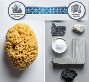
Diatoms, sea sponges, and certain plants use biological molecules and organic scaffolds to collect dissolved silicon and build complex silica structures under relatively mild conditions. The team hopes to adapt those natural processes to create lower-energy methods for breaking down silica-rich industrial waste.
The goal is not only to release rare earth elements and other critical minerals trapped inside the material, but also to convert the silica itself into useful products.
AI and Biomolecules Could Speed Discovery
The project combines expertise from biology, geochemistry, materials science, metallurgy, engineering, computational chemistry, and artificial intelligence.
Researchers plan to use advanced computational modeling and artificial intelligence to design specialized biomolecules and predict how they will interact with silicon-rich waste. These tools could help the team identify promising approaches for mineral recovery and materials manufacturing more quickly.
As lead principal investigator, Tao will manage and coordinate the overall project while also directing research on biosilicification, the process through which organisms form silica materials, and bio-enabled metallurgy for recovering rare earth elements from silicon-rich wastes.
Eggleston, a professor in the Department of Civil, Environmental, and Architectural Engineering with expertise in geochemistry, will lead work focused on understanding and optimizing the chemical reactions involved in breaking down and rebuilding silicate materials.
His research will examine reaction pathways and rates associated with silicate dissolution, repolymerization, carbonation, glass formation, and silicone synthesis.
Wang, the William B. Smith Professor of Mechanical and Materials Engineering and a widely recognized pioneer in battery recycling and sustainable manufacturing, will lead the development of bioengineered methods for recovering rare earth elements and other critical minerals.
Turning Industrial Waste Into Marketable Products
The researchers will also study whether the technologies can be scaled economically and practically for industrial use.
If the approach proves successful, it could open new ways to convert large volumes of industrial waste into marketable products. That could reduce dependence on newly mined resources, lower the environmental footprint of materials production, and strengthen domestic supplies of critical minerals and rare earth elements.
WPI graduate and undergraduate students will take part in the multiyear project through the university’s immersive STEM experience.
The effort brings together sustainability, biotechnology, materials science, data science, and artificial intelligence. It also aims to help build a broader bioengineered, silicon-based materials ecosystem by connecting researchers, industry partners, policymakers, educators, and future innovators across multiple disciplines and sectors.
Note: The above post is reprinted from materials provided by Worcester Polytechnic Institute.
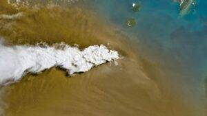
Anak Krakatau erupts ash and volcanic gases in this image acquired with the OLI (Operational Land Imager) on Landsat 8 on September 5, 2026. Credit: NASA Earth Observatory/Michala Garrison
A powerful eruption at Indonesia’s Anak Krakatau sent ash high into the atmosphere, disrupting thousands of flights and worsening air quality across parts of the country.
Anak Krakatau is a small but highly active volcano located between the Indonesian islands of Java and Sumatra. Its eruptions are often relatively modest, but the volcano is also capable of producing much more hazardous activity. In early September 2026, Anak Krakatau entered a prolonged explosive phase that lasted for more than 24 hours, sending large amounts of gas and ash into the sky. The eruption disrupted air travel and contributed to poor air quality in several areas, including Jakarta.
Satellites Capture the Eruption From Space
Satellites observed the eruption on September 5 as explosive activity continued at the volcano. One image (above), collected by the OLI (Operational Land Imager) aboard the NASA-USGS Landsat 8 satellite, shows a bright white plume of volcanic gas rising above a darker brown cloud of ash.
A broader view from the VIIRS (Visible Infrared Imaging Radiometer Suite) aboard the Suomi NPP satellite revealed volcanic material spreading across a much wider area.
By September 6, Indonesia’s meteorological agency reported that ash had climbed to altitudes of up to 6,000 meters (20,000 feet) east of the volcano and as high as 15,000 meters (50,000 feet) to the west.
Ash Cloud Disrupts Thousands of Flights
The high concentration of volcanic ash in the atmosphere forced the temporary closure of eight airports across Java and Sumatra. According to news reports, nearly 3,000 flights into and out of the affected region were disrupted.
Ash also fell over populated areas. The Indonesian Humanitarian Coordination Platform (IHCP) reported that communities east of Anak Krakatau were particularly affected, including Jakarta and other parts of West Java.
Volcanic ash can pose health concerns because it may irritate the respiratory system, eyes, and skin. The IHCP noted that the hazard differs from the smoke produced by peatland fires elsewhere in Indonesia. Volcanic ash and wildfire smoke have different particle properties, travel through the atmosphere in different ways, and require different protective measures.
Anak Krakatau Remains on High Alert
The volcano’s sustained explosive activity weakened on September 6, although Anak Krakatau continued to rumble. Its activity shifted back toward a more typical pattern of Strombolian eruptions, which involve periodic bursts of ash and other volcanic material.
Airports had resumed operation by September 8. Even so, Anak Krakatau remained at the second-highest alert level on Indonesia’s volcanic warning scale, a status it has held since early July.
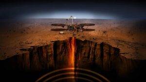
Mars hid an Earth-like geological surprise deep underground, suggesting plate tectonics may not be essential for creating complex, potentially habitable worlds. (Artist’s illustration of NASA’s InSight lander on Mars.) Credit: NASA/JPL-Caltech
Researchers at the University of Oxford have found evidence that Mars may once have contained enormous Earth-like magmatic systems deep below its surface, even though the planet does not have the plate tectonics that scientists have long associated with this level of geological complexity. The findings, published in Nature Astronomy, point to new possibilities for how rocky planets can evolve in ways that may support habitability.
Mars is commonly classified as a “stagnant lid” planet because, unlike Earth, its outer shell is not divided into moving tectonic plates. On Earth, plate tectonics plays a major role in volcanism, recycling crustal material and helping build continents. Because Mars lacks this process, scientists have often assumed that its crust formed in a much simpler way.
The new study challenges that assumption. The results suggest that Mars may have developed highly evolved crust through vigorous recycling within the planet itself, without the need for Earth-style plate tectonics.
A Mysterious Boundary 24 Kilometers Down
The researchers analyzed seismic data collected by NASA’s InSight mission, focusing on waves generated by meteoroid impacts and marsquakes, the Martian equivalent of earthquakes.
Scientists from Oxford’s Departments of Earth Sciences and Statistics used those measurements to study an unexplained boundary roughly 24 kilometers beneath the Martian surface. Earlier research had identified the boundary, but its meaning remained unclear.
To investigate whether it represented a transition between different kinds of rock, the team compared the seismic observations with hundreds of possible rock compositions. They combined thermodynamic modeling with statistical methods to determine which materials best matched the properties detected at different depths.
The analysis showed that rocks beneath the 24 km boundary were best explained by “ultramafic” material (rich in iron and magnesium, but low in silica). Above the boundary, the seismic properties were more consistent with “mafic” rocks (containing a higher proportion of silica).
Evidence of a Vast Magma System
The researchers think the buried layer formed when molten rock accumulated deep underground and gradually separated into different materials. In this process, dense crystals would have settled near the bottom of the crust, while lighter and more chemically evolved melts moved upward.
On Earth, similar processes occur beneath volcanic arcs and are associated with the formation of continents.
Lead author Dr. Tobermory Mackay-Champion (Department of Earth Sciences, University of Oxford at the time of the study, now University of Bristol) said: “We’ve traditionally assumed that volcanism on Mars was relatively simple compared to that on Earth. But this discovery suggests Mars could sustain large, long-lived systems where molten rock evolved and reprocessed itself throughout the entire crust. It raises exciting possibilities for how common such systems might be on rocky planets beyond our solar system.”
The buried layer may also be enormous in scale. According to the study, it could extend for hundreds or even thousands of kilometers across Mars’ northern hemisphere.
That would suggest ancient Mars was not dominated only by simple, isolated volcanoes. Instead, the planet may once have contained huge, connected magmatic systems spanning large portions of its crust.
This process, known as “transcrustal magmatism,” had previously been thought to be unique to Earth.
What This Could Mean for Habitable Planets
The findings could have broader implications for understanding how rocky planets become habitable.
Geological recycling can influence the development of atmospheres, oceans and environments where life might be possible. On Earth, these processes help regulate climate and support the long-term cycling of water and other volatile elements.
Because plate tectonics drives much of that recycling on Earth, scientists have often viewed it as an important requirement for creating and maintaining habitable conditions. The Mars findings suggest that complex crustal evolution and extensive geological recycling may be possible even on planets without Earth-style tectonics.
Co-author Professor Jon Wade (Department of Earth Sciences, University of Oxford) said: “One of the big questions in planetary science is whether Earth is unique. If Mars could develop this kind of complex crust without plate tectonics, then maybe the conditions needed for habitability can emerge on more planets than we realized, including those previously dismissed based on size or their apparent lack of tectonic activity.”
InSight Reveals Mars’ Hidden Interior
The research builds on seismic observations collected by NASA’s InSight mission, which placed the first seismometer on Mars in 2018 and gave scientists an unprecedented view of the planet’s internal structure.
The study was led by researchers from Oxford University’s Department of Earth Sciences in collaboration with the University of Bristol and the University of Oxford’s Department of Statistics.
Reference:
T. Mackay-Champion, M. Anderson Loake, R. Palin, J. Wade, J.-M. Kendall. Seismic evidence for a melt-depleted lower crust and transcrustal magmatism on Mars. Nature Astronomy, 2026; DOI: 10.1038/s41550-026-02907-5
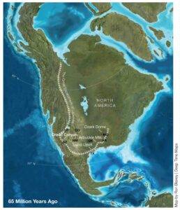
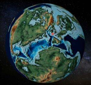
Great Escarpment of Laurentia. Map by Ron Blakey / Deep Time Maps. Credit: Prof Tom Gernon, University of Southampton
Scientists have uncovered evidence that an enormous ancient cliff system may have helped expose the deepest rocks of the Grand Canyon nearly a billion years before the Colorado River began carving the landscape seen today.
Led by researchers at the University of Southampton in the UK, the new study suggests that a vast “great escarpment” formed about 800 million years ago as the supercontinent Rodinia broke apart.
These towering cliffs may have reached roughly a kilometer in height and extended for thousands of kilometers along western North America. Over time, erosion along this immense rocky boundary removed huge amounts of material, eventually exposing ancient crystalline basement rocks that can now be seen in the Grand Canyon in southern Arizona.
A Billion Years Missing From the Grand Canyon
Thomas Gernon, Professor of Earth Science at the University of Southampton and lead author of the study, explained that the Grand Canyon preserves a geological history stretching back about two billion years. Yet more than half of that rock record appears to be absent.
He said: “Our paper suggests the Canyon’s basement rocks were progressively brought to the surface as part of an immense escarpment that developed during the breakup of an ancient supercontinent.
“The findings also shed light on the formation of the Great Unconformity, a mysterious gap in the rock record that spans over a billion years.”
Published in Geology, the research involved scientists from the University of Southampton, GFZ Helmholtz Centre for Geosciences and University of Potsdam, both in Germany, and the University of Illinois Urbana-Champaign in the USA.
The researchers propose that this ancient escarpment crossed areas that today include Arizona, Utah, Idaho, Wyoming, Colorado, Texas, Oklahoma, Arkansas, Missouri and Illinois.
Prof Gernon said powerful erosion across this enormous region eventually uncovered some of the oldest rocks in North America, with the Grand Canyon providing the best known example.
Reconstructing a Lost North American Landscape
To investigate what the region may have looked like hundreds of millions of years ago, the team combined reconstructions of plate tectonic movements with data showing how landscapes evolve through time.
Their results indicate that when Rodinia was fragmenting, the future Grand Canyon sat in roughly the same position relative to the continental edge as major escarpments found today in places such as South Africa and Brazil.
Over tens of millions of years, the giant cliff system would have gradually migrated inland as erosion wore it down. The researchers estimate that this process could have removed as much as eight kilometers of rock in some locations.
That prediction agrees with other geological evidence showing that roughly five to ten kilometers of rock disappeared from parts of the region long before the modern Grand Canyon formed.
“This long-lived tectonic landscape provides a missing piece in understanding why erosion associated with the Great Unconformity varies so dramatically across the southwestern US,” said Prof Gernon.
He added: “Our work suggests that tectonic uplift related to continental rifting and breakup created both steep slopes and high ground, providing the mountainous terrain that rivers and glaciers could readily erode.”
An Ancient Mountain Rim That Reshaped North America
The influence of this enormous escarpment may have extended far beyond the area that eventually became the Grand Canyon.
By producing a long-lived mountainous rim around western Laurentia — the ancient core of North America — the landscape may have shaped the paths of rivers, determined where sediments collected, and influenced when rising seas spread across the continent before the so-called Cambrian explosion, a period when complex life diversified rapidly.
Prof Gernon added: “Today’s escarpments in Africa, Brazil, India and Antarctica provide windows into the forces that shape continents over hundreds of millions of years.
“By comparing Grand Canyon’s ancient history with active landscapes like the Great Escarpment of South Africa, we’re able to see North America’s most iconic geologic landmark in an entirely new light.
“Our findings could help geologists reinterpret other ancient continental interiors where similarly large gaps occur in records, offering a better understanding of how Earth’s continents have changed over hundreds of millions of years.”
Reference:
Thomas M. Gernon, Thea K. Hincks, Elias J. Rugen, Sascha Brune, Jean Braun, Stephen Marshak. Exhumation of Grand Canyon’s basement along the Great Escarpment of Laurentia. Geology, 2026; DOI: 10.1130/G55133.1
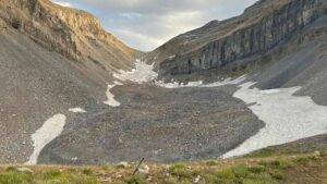
This cirque under Utah’s Mount Timpanogos contains a hidden ‘rock glacier’ holding enough water to fill 600 Olympic swimming pools, according to University of Utah researchers. Credit: Bronson Cvijanovich, University of Utah
Rock glaciers look very different from conventional glaciers. Instead of exposed ice, they resemble sprawling fields of loose rock, while potentially concealing large quantities of ice below the surface. These formations are widespread across Utah’s Wasatch and Uinta ranges and can also be found on the Colorado Plateau in the La Sal Mountains near Moab.
University of Utah geologists have now taken a detailed look inside one of the state’s largest examples, the Timpanogos Rock Glacier beneath the prominent summit of Mount Timpanogos near Salt Lake City and Provo. Two new studies examine how the glacier formed and reveal how much ice is buried inside it. By detecting extremely small differences in the gravitational pull of rock and ice, the researchers developed a new way to create a 3D image of the hidden ice within a large rock glacier.
The results show that Timpanogos Rock Glacier contains about 1.5 million cubic meters of frozen water, enough to fill roughly 600 Olympic swimming pools. Bronson Cvijanovich, a former graduate student in the Department of Geology & Geophysics, noted that this is also about the same volume as the largest pyramid at Giza in Egypt.
“Timpanogos Rock Glacier is surprisingly ice rich. It is 83% ice and 17% loose rock,” said Cvijanovich, lead author of one of the two studies overseen by geophysics professor Michael Thorne and glaciology professor Leif Anderson.
Hidden Ice Beneath Mount Timpanogos
“There’s a lot of ice that’s hidden in Utah’s mountains,” Anderson said. “When we are high in the mountains and walking across loose rocks or rubble, you don’t realize there could be 120 feet of ice buried beneath your feet.”
During the fall of 2024, Cvijanovich led a series of field trips to Timpanogos Rock Glacier, carrying sensitive equipment to the buried ice above Emerald Lake. Among the instruments was a state-of-the-art gravimeter. Across six trips, he collected gravity measurements at 232 locations arranged in a grid across the glacier, with each point separated by 25 meters (~80 feet).
A gravimeter can detect differences in density, allowing researchers to distinguish the denser surrounding rock from the much lighter buried ice. Those measurements can then be used to estimate the shape and thickness of the hidden glacier.
“There is a large contrast in mass density between the rock that makes up Mount Timpanogos and the much lower density ice that is in rock glacier adjacent to it,” Thorne said. “When we measure the gravitational acceleration over the rock glacier, we see a larger decrease in that gravitational acceleration as we make measurements over areas with thicker ice.”
Building a 3D View With Gravity
Collecting the gravity data was only the first step. The researchers also had to account for subtle changes caused by the positions of the sun and the moon, as well as differences in terrain, latitude, and elevation.
After making those corrections, the team developed a new method for reconstructing the glacier’s internal ice in three dimensions using Bayesian statistics. “We spent months of computation time doing the imaging with our new techniques,” Thorne said.
Satellite images can show the surface footprint of a rock glacier, but they provide much less information about its depth, internal structure, and total amount of buried ice. Measuring those features requires instruments capable of revealing what lies beneath the rubble, similar to how a CT scanner can reveal bones and tissues inside the human body.
How Utah’s Rock Glaciers Form
Rock glaciers commonly develop beneath steep mountain valleys or cirques where falling debris regularly collects. In the Wasatch Mountains, that falling material appears to play a key role in protecting snow from melting.
“In the Wasatch, the mountains themselves are eroding and burying the snow, and that’s why the rock glaciers exist,” Anderson noted.
The researchers developed a new mathematical model describing how these glaciers grow. Their results suggest that rockfalls repeatedly cover persistent snow in the upper sections of rock glaciers, adding mass and helping preserve the snow beneath layers of debris.
The second study also indicates that Utah’s rock glaciers are not leftover features from the Ice Age (which reached its peak 21,000 to 18,000 years ago). Instead, they are reservoirs of frozen water that developed during the thousands of years after the major Ice Age glaciers disappeared.
A Potentially Huge Mountain Water Reserve
Timpanogos Rock Glacier is one of 836 rock glaciers identified across Utah through satellite imagery. Using the detailed measurements from Timpanogos, the researchers established a relationship between a rock glacier’s surface area and the volume of ice stored underneath it.
They then applied that relationship more broadly. Their calculations suggest that the roughly 50,000 known rock glaciers around the world could collectively contain about 48 gigatons of water. Equal to 1 billion metric tons, a gigaton is the equivalent of a cubic kilometer of water, enough to fill 400,000 Olympic swimming pools.
Within Utah alone, rock glaciers may contain about 1 gigaton of water, or approximately 815,000 acre-feet, according to the researchers.
Two Studies Examine Utah’s Hidden Ice
The research titled “The internal ice content of Timpanogos Rock Glacier, Utah, USA from 3-D Bayesian inversion of gravity data,” was published Aug. 26 in the Journal of Geophysical Research.
The earlier paper, “Mass Addition to Timpanogos Rock Glacier: Debris‐ Covered Snow and the Importance of Interannual Variability in Headwall Erosion and Climate,” appeared in Geophysical Research Letters on April 2, 2026. Isaiah Davies, an undergraduate at Stanford University and visiting summer researcher at the University of Utah in 2023, was the lead author.
The research was supported by the U.S. Geological Survey, National Science Foundation, University of Utah’s Wilkes Center for Climate Science & Policy, the U’s Office of Undergraduate Research, and the Summer Program for Undergraduate Research.
Reference:
Bronson Cvijanovich, Michael S. Thorne, Surya Pachhai, Leif S. Anderson, Ivan Tochimani‐Hernandez, Christian L. Hardwick, Tonie van Dam. The Internal Ice Content of Timpanogos Rock Glacier, Utah, USA From 3‐D Bayesian Inversion of Gravity Data. Journal of Geophysical Research: Earth Surface, 2026; 131 (8) DOI: 10.1029/2026jf009214
Note: The above post is reprinted from materials provided by University of Utah. Original written by Brian Maffly.
Green hydrogen can be generated using Western Australia’s vast iron-ore deposits. Credit: Edith Cowan University
Researchers at Edith Cowan University (ECU) have identified a potentially important source of low-emission energy beneath Western Australia, where vast iron-rich formations may be capable of generating naturally occurring hydrogen.
The findings suggest that the region’s geology could eventually support a new domestic energy source and, if developed at scale, a major hydrogen export industry.
Magnetite Could Generate Hydrogen Underground
The research focuses on magnetite, a mineral that is abundant in Western Australia’s huge iron ore deposits across the Pilbara region.
Scientists from ECU’s School of Engineering found that magnetite can release hydrogen gas when it reacts with hot water under conditions similar to those deep below the Earth’s surface.
The team also discovered a way to stimulate the process. By injecting a solution into banded iron formations, the researchers were able to increase hydrogen generation, raising the possibility that naturally produced hydrogen could one day be deliberately enhanced underground.
“Australia could be sitting on a massive, untapped energy reserve — and the potential is enormous,” Associate Professor Alireza Keshavarz said.
“There is enough hydrogen for Australia to benefit for generations, and potentially enough for us to become a major exporter of clean energy to the rest of the world.”
Recreating Deep Underground Conditions
To investigate how the process works, the researchers placed magnetite samples in water at 200°C under high pressure for 60 days. Those conditions were designed to reproduce the hot, pressurized environment found deep underground.
The experiments gave researchers a clearer picture of how natural hydrogen can form within rock and what conditions are needed for production to continue over time.
The findings are especially significant for Western Australia because the region contains some of the largest banded iron formations on Earth.
“Western Australia has some of the world’s largest banded iron formations. If we can unlock this resource at scale, it could be transformative for our energy future,” lead author Kaveh Moghanirahimi said.
“We even see the potential for Western Australia to strengthen its energy independence during times of crisis through access to this naturally generated hydrogen.”
From Laboratory Experiments to Natural Hydrogen Exploration
Professor Stefan Iglauer, from ECU’s School of Engineering, said the results bring researchers closer to understanding how hydrogen production might work in real underground rock formations rather than only in controlled laboratory settings.
“This work helps bridge the gap between laboratory experiments and real geological systems,” Professor Iglauer said.
The study also found that the amount of magnetite alone does not determine how much hydrogen can be produced. The structure of the rock matters as well, particularly whether water can move through it and reach fresh mineral surfaces.
“Our findings show that hydrogen production depends not only on the amount of magnetite present, but also on how easily water can access fresh mineral surfaces through fractures, pores and permeable pathways.”
That means fractures, pores, and other pathways through the rock could play a critical role in determining whether natural hydrogen can be generated efficiently enough to become a practical energy resource.
The research, Geometry-driven controls on hydrothermal natural hydrogen generation from magnetite mineral, has been published in the International Journal of Hydrogen Energy.
Reference:
Kaveh Moghanirahimi, Lionel Esteban, Valeriya Shulakova, Muhammad Ali, Stefan Iglauer, Alireza Keshavarz. Geometry-driven controls on hydrothermal natural hydrogen generation from magnetite mineral. International Journal of Hydrogen Energy, 2026; 220: 154187 DOI: 10.1016/j.ijhydene.2026.154187
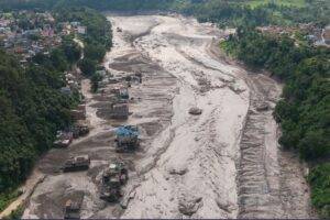
A drone view shows mud covering properties following a flash flood at Trishuli in Nuwakot district, Nepal, on Wednesday. Stringer/Reuters
On August 26, 2026, a catastrophic flash flood swept through the Himalayan border region of Nepal and Tibet, causing severe destruction along the Lhende Khola–Bhote Koshi–Trishuli river system. Settlements, roads, bridges, hydropower infrastructure, and sections of the trans-Himalayan transport corridor were damaged or destroyed, while rescue operations continued amid extensive loss of life and large numbers of missing people.
The disaster was unusual because available hydrological evidence does not support an intense local rainstorm as its primary trigger. Nepal’s Department of Hydrology and Meteorology reported that there had not been heavy rainfall in the affected Rasuwa area immediately before the flood. Instead, satellite imagery, seismic observations, and preliminary assessments point toward a large high-altitude ice-rock mass movement that entered the Lhende Khola catchment and initiated a cascading sequence of processes.
Satellite imagery reviewed by scientists indicates that a substantial portion of the lower part of a glacier detached at approximately 5,200 metres elevation and descended roughly 1,200 vertical metres toward the valley floor. The collapsing ice appears to have entrained rock and sediment, creating an ice-rock avalanche rather than a simple fall of clean glacier ice.
Preliminary satellite analysis by Nepal’s Department of Hydrology and Meteorology further suggests that the avalanche and associated debris may have temporarily blocked the river about 20 km upstream of the Miteri Bridge, producing an impoundment that subsequently released water downstream. This river-blockage interpretation is plausible and supported by early imagery, but it remains a preliminary reconstruction rather than a fully resolved post-event model.
The Nepal flash flood of August 2026 is therefore best understood, at present, as a cascading cryospheric and geomorphic disaster: an initial glacier or ice-rock instability generated a large mass movement, the mass movement interacted with the river system, water and sediment were rapidly mobilized, and the resulting flood transformed as it moved through steep Himalayan valleys.
This distinction is important. The event was not simply “a glacier melting” and it should not yet be described uncritically as a conventional glacial lake outburst flood. Its destructive power appears to have emerged from the interaction of ice, rock, water, steep relief, temporary river obstruction, sediment entrainment, and confined valley geometry.
What Caused the August 2026 Nepal Flash Flood?
The Initial Ice-Rock Avalanche
The best available evidence indicates that the disaster began with the failure of a high-altitude glacier or glacier-associated slope in the Langtang–Nepal/Tibet border region.
Before-and-after Planet Labs imagery showed a major change in the source area. Researchers examining the images identified a substantial collapse from the lower glacier, followed by extensive deposits of fragmented ice, rock, and sediment on the valley floor. Reuters reported that Nepal’s National Disaster Risk Reduction and Management Authority described the event as a glacier-involved flood associated with a snow-rock or ice-rock mass movement in the upper Lhende drainage.
An ice-rock avalanche is a rapid gravitational mass movement containing substantial quantities of both glacier ice and rock debris. Such events can be extraordinarily mobile because fragmentation, ice deformation, entrained water, snow, and fine sediment reduce internal resistance during movement.
The physical process begins with gravitational potential energy:
Ep=mghE_p = mgh
where:
EpE_p is gravitational potential energy
mm is the mass of unstable material
gg is gravitational acceleration
hh is the vertical drop
For the August 2026 event, the reported vertical fall of approximately 1.2 km implies an enormous potential-energy release. However, a defensible event-specific energy calculation cannot yet be made because the three-dimensional failure volume, average thickness, rock-to-ice ratio, density, and entrained mass remain insufficiently constrained.
This is an important scientific limitation. Mapping the surface area of a collapse scar is not equivalent to determining the volume or mass of the failed material.
From Glacier Failure to a Valley-Scale Mass Flow
Once ice and rock began accelerating downslope, the moving avalanche likely fragmented and entrained additional material from the slope and valley floor.
Possible entrained materials include:
unconsolidated glacial sediment
moraine debris
talus
weathered bedrock
snow
channel sediment
and river water
The result can be a rapidly evolving multiphase flow whose behavior changes with distance.
A comparable process was documented during the 2021 Chamoli disaster in the Indian Himalaya, when approximately 27 million m³ of rock and glacier ice collapsed and transformed into an exceptionally mobile debris flow. Shugar et al. (2021) showed that entrainment and flow transformation were fundamental to the downstream disaster. The Chamoli event should not be treated as an exact analogue for the 2026 Nepal flood, but it demonstrates the physical plausibility of an ice-rock avalanche evolving into a highly destructive valley-confined flow.
How River Blockage May Have Amplified the Disaster
Formation of a Temporary Natural Dam
One of the most significant findings in the preliminary reconstruction is evidence that ice and debris may have blocked the river.
Nepal’s Department of Hydrology and Meteorology reported that satellite images supplied by Chinese authorities showed a blockage approximately 20 km upstream of the Miteri Bridge. Officials interpreted the images as showing an icefall or landslide, formation of an impounded water body behind debris, and subsequent release.
A temporary blockage produced by an avalanche is known as a landslide dam, avalanche dam, or, where glacier ice is an important component, an ice-debris dam.
Unlike an engineered dam, such barriers are highly heterogeneous. They may contain a poorly sorted mixture of:
boulders
fractured bedrock
gravel
sand
silt
snow
glacier ice
and organic material
Their internal permeability and mechanical strength can vary dramatically over very short distances.
Why Temporary Landslide Dams Can Fail Rapidly
Water accumulating behind an avalanche deposit increases hydrostatic loading on the barrier. Failure may occur through several mechanisms, including overtopping, erosion of the downstream face, piping through permeable sediment, internal collapse, melting of ice-rich portions, or progressive channel incision.
Once overtopping begins, flowing water can rapidly erode an unconsolidated dam. As the breach deepens and widens, discharge rises, which accelerates erosion still further.
This positive feedback can generate an abrupt flood wave.
For the August 2026 event, the temporary-dam hypothesis is strongly supported by preliminary satellite interpretation, but researchers still need to determine the dimensions of the blockage, duration of impoundment, volume of stored water, breach mechanism, and relative contribution of other water sources.
Was the Nepal Flash Flood Caused by an Earthquake?
The Early Earthquake Interpretation
During the first hours after the disaster, a seismic signal detected near the Nepal–Tibet border was reported as a magnitude 4.4 earthquake. This immediately raised the possibility that tectonic shaking had destabilized the glacier or slope.
That interpretation changed as more data became available.
The U.S. Geological Survey subsequently revised the event, concluding that the seismic energy was generated by the glacier collapse and associated debris movement rather than by tectonic fault rupture. Reports based on the USGS reassessment state that the source was revised to a seismic magnitude of about 5.2 and classified as a glacial collapse/debris-flow event rather than an earthquake.
This distinction is fundamental.
A magnitude assigned to a seismic source describes the size of the recorded seismic signal; it does not automatically mean that the source was an earthquake produced by fault slip.
How Seismologists Distinguish Landslides from Earthquakes
Large landslides, rock avalanches, and glacier collapses can generate seismic waves detectable hundreds or even thousands of kilometres away.
The source physics, however, differs from that of a conventional tectonic earthquake.
In a typical tectonic earthquake, elastic strain is suddenly released by slip on a fault. The seismic source is commonly represented by a double-couple moment tensor.
A large landslide or avalanche instead produces ground forces as a moving mass accelerates, interacts with topography, changes direction, impacts the valley floor, and decelerates. For sufficiently large events, these dynamics can often be approximated using time-dependent single-force or centroid-force models.
Ekström and Stark (2013) demonstrated that long-period seismic waves produced by very large landslides can be inverted to estimate properties such as the duration, momentum, direction, potential-energy loss, and approximate mass of the moving material.
Scientists therefore do not identify a glacier collapse using one simple signal characteristic. Instead, they integrate seismic waveform and spectral behavior, arrival characteristics, long-period source modeling, event location, and independent geomorphic observations such as satellite imagery.
For the August 2026 event, reports indicate that the USGS reassessment incorporated data from nearby seismic stations, long-period seismic observations, and satellite evidence.
This multi-dataset approach is more robust than interpreting the seismic magnitude alone.
Was the August 2026 Event a Glacial Lake Outburst Flood?
What Is a GLOF?
A glacial lake outburst flood, commonly abbreviated GLOF, occurs when water stored in a glacier-related lake is released suddenly.
The lake may be dammed by:
moraine
glacier ice
bedrock
landslide debris
or combinations of these materials
A GLOF can be triggered by an ice avalanche entering a lake, rockfall, moraine failure, intense rainfall, rapid snowmelt, earthquake shaking, internal piping, or progressive instability.
Why the Classification of the 2026 Flood Requires Caution
Calling the August 2026 Nepal event a conventional GLOF may be premature.
Early investigations considered whether a pre-existing glacial lake had burst, partly because the region contains glacial lakes and has experienced previous outburst floods. However, the more recent preliminary reconstruction emphasizes an ice-rock avalanche followed by river blockage and temporary impoundment. Nepalese officials have stated that whether an additional glacial lake outburst occurred remains under investigation.
At present, the most scientifically cautious terminology is:
an ice-rock-avalanche-triggered cascading flash flood, potentially involving temporary river damming and outburst.
If later investigations demonstrate that the dominant floodwater originated from a pre-existing glacier-fed lake, classification as a GLOF would become more appropriate.
If instead the main reservoir formed only after avalanche debris blocked the river, the process would be more accurately described as an avalanche-dammed or landslide-dam outburst flood.
The distinction is not semantic. Different mechanisms require different monitoring strategies.
Why Was the Flood So Destructive?
Extreme Himalayan Relief
The Himalaya provides ideal topographic conditions for rapid conversion of gravitational potential energy into destructive mass movement.
The suspected source material fell approximately 1,200 vertical metres from the glacier toward the valley below. Such relief allows an avalanche to accelerate rapidly before reaching the channel system.
Once the moving mass enters a narrow valley, it can maintain substantial momentum while simultaneously entraining sediment and water.
Sediment Entrainment and Flow Bulking
A flood originating upstream does not necessarily maintain a constant volume as it travels downstream.
In steep mountain channels, energetic flows can erode:
channel banks
river terraces
alluvium
landslide deposits
moraines
road embankments
and previously deposited debris
This process is known as entrainment or bulking
As more sediment becomes incorporated, the flow may increase in density and destructive power.
The preliminary Nepalese assessment specifically noted that the large quantity of sediment transported with the flood substantially increased its destructive effect compared with a clear-water flood.
Transition Between Flood and Debris-Flow Behavior
Mountain floods exist along a continuum.
At relatively low sediment concentrations, the flow behaves predominantly as turbulent water. As sediment concentration increases, interactions between particles become increasingly important.
These categories should not be assigned to the August 2026 event without quantitative sediment-concentration measurements, but imagery clearly indicates that the surge transported large quantities of mud, rock, and boulders.
Such sediment-rich flows can exert enormous impact forces on bridges, hydropower structures, buildings, and retaining walls.
Why Did the Flood Remain Powerful Far Downstream?
Channel Confinement
The Bhote Koshi and upper Trishuli systems pass through steep, confined Himalayan valleys.
In a broad floodplain, floodwater can spread laterally, reducing depth and velocity. In a narrow gorge, the same discharge is concentrated into a much smaller cross-sectional area.
This confinement can maintain high flow velocities and depths for substantial distances.
Rapid Flood-Wave Propagation
Hydrological observations illustrate the unusual speed of the August 2026 surge.
According to ICIMOD information reported by Reuters, water levels at Galchhi on the Trishuli River rose by as much as approximately nine metres within about 30 minutes.
Such a rapid change is consistent with an abrupt upstream release rather than slowly developing rainfall runoff.
The flood also propagated through the Bhote Koshi into the Trishuli system and altered river corridors well downstream from its source.
Why the Lhende–Bhote Koshi Region Is Particularly Hazardous
Active Tectonics and Extreme Relief
The Himalaya exists because of the ongoing convergence between the Indian and Eurasian plates.
Continued crustal shortening and uplift, combined with rapid river incision, maintain very high topographic relief. The resulting landscape contains steep slopes, deeply incised valleys, fractured bedrock, and large volumes of unconsolidated sediment.
These conditions naturally favor:
landslides
rock avalanches
debris flows
glacier avalanches
river blockage
and catastrophic sediment transport
This does not mean tectonic activity directly triggered the August 2026 collapse. Rather, tectonics creates the steep and mechanically complex landscape in which such gravitational hazards occur.
Cryospheric Instability
High Himalayan valleys contain glaciers, seasonal snow, permafrost, moraines, and glacier-fed lakes. These components respond differently to temperature, precipitation, and long-term climate change.
A destabilized glacier can therefore interact with an unstable slope, a river, or a lake to create compound or cascading hazards.
The 2026 disaster illustrates why hazard assessment cannot treat glaciers, landslides, and floods as independent processes.
Previous Glacier-Related Floods in the Central Himalaya
The Poiqu–Bhote Koshi Transboundary Hazard Corridor
The broader central Himalayan border region has a documented history of glacier-related flooding.
Wang et al. (2024) reconstructed the 2002 Poiqu No. 1 GLOF and the 2016 Gongbatongsha Co GLOF in the transboundary Poiqu River basin. Their analysis showed that ice avalanches were the dominant triggers for both events and that the resulting floods underwent complex downstream flow transformations.
This is directly relevant to the August 2026 disaster because it demonstrates that ice avalanches can serve as the first stage of destructive transboundary flood cascades in the central Himalaya.
The historical events do not prove the precise mechanism of the 2026 flood, but they provide an important geological framework for understanding the region’s susceptibility.
Lessons from the 2021 Chamoli Disaster
The 2021 Chamoli event provides another useful comparison.
Shugar et al. documented how a large rock-and-ice avalanche transformed into a highly mobile debris-rich flow that devastated downstream hydropower infrastructure. The study demonstrated how a hazard beginning on a remote high-altitude slope can rapidly evolve into a completely different process downstream.
The key lesson is that hazard classification at the source does not necessarily describe the hazard experienced downstream.
An ice avalanche can become a debris flow.
A landslide can form a dam.
A temporary lake can generate an outburst flood.
A flood can entrain enough sediment to acquire debris-flow-like characteristics.
This process chain is what geologists mean by a cascading hazard.
Did Climate Change Cause the Nepal Flash Flood?
What We Know About Himalayan Glacier Change
There is strong scientific evidence that Himalayan glaciers have undergone substantial mass loss during recent decades.
Maurer et al. (2019), using historical satellite imagery and modern digital elevation models across a roughly 2,000-km Himalayan transect, found that average glacier ice-loss rates approximately doubled between 1975–2000 and 2000–2016, consistent with regional atmospheric warming as the dominant large-scale driver.
Climate-driven changes can modify high-mountain hazards through several physical pathways:
glacier thinning
changing glacier geometry
increased meltwater production
changing subglacial water pressure
loss of ice support from valley walls
permafrost degradation
changing freeze–thaw conditions
and growth or formation of glacier-fed lakes
These mechanisms make a climatic influence on Himalayan slope and glacier stability scientifically plausible.
Why Event Attribution Requires More Evidence
However, there is an important difference between saying that climate change modifies the regional hazard environment and claiming that it directly caused one particular collapse.
The exact trigger of the August 2026 initial failure remained under investigation on August 27. Scientists quoted by Reuters cautioned against attributing the collapse to climate change as a single immediate cause.
Possible controlling factors include glacier geometry, bed conditions, meltwater pressure, rock structure, snow conditions, preceding temperature, progressive deformation, and other local processes.
Some of these variables may themselves be influenced by long-term warming, but a scientifically defensible attribution requires event-specific evidence.
The safest conclusion is therefore:
Climate change is altering the physical conditions of the Himalayan cryosphere and can increase susceptibility to some glacier and slope failures, but the specific causal contribution of climate change to the August 2026 collapse has not yet been quantified.
What Previous Glacier Collapses Tell Us
The possibility of climate and hydrological forcing influencing glacier collapse is well established scientifically.
Kääb et al. (2018) investigated two enormous glacier collapses in western Tibet in 2016. They found that climate- and weather-related forcing interacted with unusual glacier-bed properties, subglacial water, and glacier dynamics to produce catastrophic failure.
This demonstrates that climate can be one component of a glacier-instability mechanism without functioning as a simple, isolated trigger.
That distinction should also guide interpretation of the 2026 Nepal flood.
The Role of Permafrost and Rock-Slope Instability
Frozen Ground as Part of Mountain Strength
High mountain bedrock commonly contains fractures filled with ice.
Where permafrost is present, ice within fractures can contribute to the mechanical behavior of rock slopes. Warming and thawing may change fracture-water pressure, reduce ice bonding, and promote progressive rock-mass instability.
However, the presence, depth, and thermal state of permafrost at the exact 2026 source zone have not yet been sufficiently documented to claim that permafrost degradation triggered the event.
It should therefore be treated as a possible regional process, not an established event-specific cause.
Glacier Debuttressing
As glaciers thin or retreat, they can expose valley walls that were previously in contact with glacier ice.
This process is commonly termed debuttressing.
The mechanical importance of glacier buttressing differs greatly between sites. Retreat does not automatically produce slope failure, but changing boundary conditions may contribute to long-term instability in already fractured mountain slopes.
Again, whether this process was important in the August 2026 source area remains to be tested.
What Satellite Imagery Reveals About the Disaster
Mapping the Source Scar
High-resolution satellite imagery is especially important in remote Himalayan disasters because the source area may be inaccessible for days or weeks.
Before-and-after imagery can identify:
newly exposed failure scars
missing glacier sections
avalanche deposits
newly formed lakes
channel blockages
sediment fans
altered river courses
and downstream inundation
Planet Labs imagery provided some of the first strong evidence that a major glacier-associated collapse had occurred during the August 2026 event.
Why Satellite Imagery Must Be Combined With Other Data
Satellite imagery alone cannot fully determine:
the exact timing of failure
the total avalanche volume
water discharge
subsurface conditions
dam-breach dynamics
or the complete sequence of events
A robust reconstruction therefore combines remote sensing with:
seismic records
river-stage measurements
digital elevation models
field mapping
sedimentological evidence
eyewitness videos
and numerical flow models
This multidisciplinary strategy was successfully used after the 2021 Chamoli event and in reconstructions of previous central Himalayan GLOFs.
What Geological Evidence Will Researchers Look for Next?
Source-Area Reconstruction
Scientists will need high-resolution topographic data to calculate the true three-dimensional geometry of the failed glacier and slope.
Comparing pre- and post-event digital elevation models can constrain:
failure volume
ice-versus-rock proportions
vertical displacement
erosion
and deposit thickness
These values are necessary for credible energy and mass-balance calculations.
Sedimentological Evidence
Downstream deposits can reveal how the flow changed with distance.
Geologists will examine:
grain-size distributions
boulder imbrication
matrix-supported versus clast-supported textures
scour surfaces
mud drapes
high-water marks
channel erosion
and sediment thickness
These observations can help distinguish sections dominated by debris flow, hyperconcentrated flow, and conventional flooding.
Evidence of Temporary Damming
If a temporary landslide dam controlled the flood, researchers should be able to identify geomorphic evidence such as:
remnants of the blockage
upstream sediment or water-level marks
a breach channel
erosional scarps
lacustrine sediment
and post-event channel reorganization
This evidence will be critical for determining whether the early dam-outburst interpretation is correct.
Can Similar Himalayan Flash Floods Be Predicted?
Hazard Identification Is Easier Than Exact Prediction
Scientists can identify unstable glaciers and potentially dangerous slopes, but predicting the exact time of catastrophic failure remains extremely difficult.
Possible indicators include:
accelerating glacier motion
widening crevasses
progressive slope deformation
growth of supraglacial ponds
changing drainage pathways
increasing rockfall
unstable moraine dams
and anomalous seismic activity produced by cracking or mass movement
No individual signal guarantees that failure will occur.
Monitoring Must Extend Beyond Glacial Lakes
Traditional Himalayan cryospheric hazard programs have often focused heavily on identifying large glacial lakes.
That remains essential, but events such as Chamoli and the preliminary reconstruction of the August 2026 Nepal flood demonstrate that catastrophic floods can originate without the straightforward failure of a previously mapped large lake.
Monitoring strategies should therefore include:
hanging glaciers
steep glacier termini
ice-rock avalanche source zones
permafrost slopes
landslide dams
supraglacial lakes
glacier drainage systems
and downstream sediment stores
The key concept is source-to-river connectivity.
Why Transboundary Monitoring Is Essential
Flood Basins Ignore Political Borders
The August 2026 disaster affected both Nepal and Tibet and propagated through a river system crossing politically sensitive mountainous terrain.
Upstream mass movements can generate downstream hazards before communities have enough time to understand what happened.
Effective warning therefore depends on rapid exchange of:
seismic information
river-gauge data
satellite observations
glacier monitoring
meteorological measurements
and reports of upstream blockage
The transboundary nature of previous Poiqu–Bhote Koshi GLOFs makes this need particularly clear.
Cascading-Hazard Warning Systems
A conventional flood warning system may detect rising river levels only after a catastrophic release has begun.
A more advanced system would integrate multiple sensors.
For example, a large mass movement detected seismically could automatically trigger analysis of satellite imagery and downstream river gauges. If both an avalanche signal and sudden river-stage rise were detected, alerts could be issued to communities farther downstream.
Such integrated systems are increasingly important in steep glacierized mountain regions.
Frequently Asked Questions About the August 2026 Nepal Flash Flood
What caused the Nepal flash flood in August 2026?
The best available evidence indicates that a large ice-rock avalanche associated with the collapse of part of a high-altitude glacier initiated the disaster. Preliminary satellite analysis also suggests that debris temporarily blocked the Lhende river system, allowing water to accumulate before a sudden downstream release. The detailed sequence is still being investigated.
Was an earthquake responsible for the flood?
Current USGS interpretation indicates no tectonic earthquake triggered the event recorded by its network. A signal initially catalogued as a magnitude 4.4 earthquake was subsequently reinterpreted as seismic energy generated by the glacier collapse and debris movement, with the source revised to approximately magnitude 5.2.
Does magnitude 5.2 mean there was a magnitude 5.2 earthquake?
No. Seismic magnitude does not by itself identify the physical source as an earthquake. Very large landslides and glacier collapses can generate strong seismic signals. Source modeling and independent geological evidence are needed to determine whether the signal resulted from fault rupture or gravitational mass movement.
Was the event a GLOF?
Possibly in a broad glacier-related sense, but a conventional pre-existing glacial lake outburst has not yet been conclusively demonstrated. The strongest current preliminary interpretation involves an ice-rock avalanche and temporary river blockage. It is therefore safer to describe the disaster as an ice-rock-avalanche-triggered cascading flood pending detailed investigation.
Did heavy rainfall cause the flood?
Heavy local rainfall does not currently appear to have been the primary trigger. Nepal’s Department of Hydrology and Meteorology reported that substantial rainfall had not occurred in the Rasuwa area immediately before the disaster.
Did climate change cause the glacier collapse?
The answer is not yet known. Climate warming is clearly driving major glacier changes across the Himalaya and can modify conditions controlling glacier and slope stability. However, determining how much climate change contributed to this specific collapse requires detailed event attribution.
Why was the flood carrying so much mud and rock?
The initial mass movement supplied large quantities of debris, while the high-energy downstream flow could also erode and entrain additional sediment from channels, riverbanks, terraces, and existing slope deposits. Preliminary observations indicate that sediment and boulders were a major component of the destructive surge.
What the August 2026 Nepal Flood Teaches Us About Himalayan Geology
The central scientific lesson from the disaster is that extreme Himalayan floods often cannot be explained by a single process.
The current evidence points toward a sequence resembling:
glacier or ice-rock instability → catastrophic mass movement → river interaction → probable temporary obstruction → rapid water release → sediment entrainment → debris-rich flood → downstream geomorphic transformation
Each stage can amplify the next.
This is why the term cascading geohazard is so important.
The August 2026 Nepal flash flood demonstrates that a failure beginning high on an isolated mountain slope can propagate through the landscape and become a regional hydrological disaster.
It also demonstrates why geological hazards cannot always be neatly separated into categories such as “landslide,” “glacial hazard,” and “flood.”
In steep mountain systems, they are dynamically connected.
References
Shugar, D. H., Jacquemart, M., Shean, D., et al. (2021). A massive rock and ice avalanche caused the 2021 disaster at Chamoli, Indian Himalaya. Science, 373(6552), 300–306. doi: 10.1126/science.abh4455.
Kääb, A., Leinss, S., Gilbert, A., et al. (2018). Massive collapse of two glaciers in western Tibet in 2016 after surge-like instability. Nature Geoscience, 11, 114–120. doi: 10.1038/s41561-017-0039-7.
Maurer, J. M., Schaefer, J. M., Rupper, S., & Corley, A. (2019). Acceleration of ice loss across the Himalayas over the past 40 years. Science Advances, 5(6), eaav7266. doi: 10.1126/sciadv.aav7266.
Ekström, G., & Stark, C. P. (2013). Simple scaling of catastrophic landslide dynamics. Science, 339(6126), 1416–1419. doi: 10.1126/science.1232887.
Wang, X., Zhang, G., Veh, G., Sattar, A., Wang, W., Allen, S. K., Bolch, T., Peng, M., & Xu, F. (2024). Reconstructing glacial lake outburst floods in the Poiqu River basin, central Himalaya. Geomorphology, 449, 109063. doi: 10.1016/j.geomorph.2024.109063.
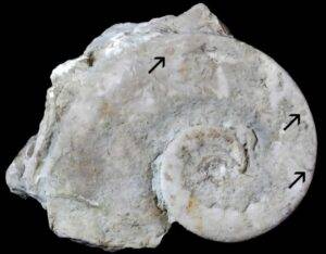
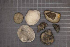
Steinkern of Maclurites neritoides containing cryptic fauna cornulitids, bryozoans, and graptolites (arrows). Credit: Scientific Reports (2026). DOI: 10.1038/s41598-026-62638-5
An international study led by researchers from the University of Tartu shows that approximately 470 million years ago, a significant ecological change took place in the world’s oceans: For the first time, the interiors of empty mollusk shells began to be used as habitats. This marked the emergence of a new ecological niche and was a crucial step in the development of a marine ecosystem similar to today’s.
In modern seas, empty mollusk shells rarely remain unoccupied for long. They are often covered with various attached invertebrates, such as bryozoans and annelids. However, the study shows that during the Cambrian Period, more than 500 million years ago, the interiors of such shells remained completely uninhabited, even though organisms living in sheltered cavities already existed.
A team of researchers, including Olev Vinn, Oive Tinn, Liisa Lang and Mare Isakar from the University of Tartu, analyzed fossils from different parts of the world and found that the first animals to colonize these sheltered habitats appeared in mollusk shells during the Middle Ordovician, or about 460 million years ago. Initially, the relatively large and spacious shells of cephalopods—or nautiloids—were colonized, and later, these small inhabitants also spread into the interiors of snails and clams. Their paper is published in the journal Scientific Reports.
By the Late Ordovician—about 450 million years ago—the interiors of many shells were already densely covered with attached fauna. These were inhabited by animals that filtered food particles floating in the water, such as bryozoans, brachiopods, sponges, graptolites and cornulids, which built tube-shaped shells.
However, not all empty shells provided the same living conditions. The study revealed that although the communities living in the shells of snails, clams and cephalopods were quite similar in terms of species composition, the shape of the shells influenced how numerous the organisms were and how large they grew. Water circulated more freely in the spacious chambers of the nautiloids, supplying the animals with oxygen and food and carrying away metabolic waste. Consequently, it is precisely in these shells that the most diverse fossil communities are found.
In the coiled shells of snails with narrow openings, water exchange was poorer, and the organisms that grew there were mostly smaller; moreover, some animal groups requiring a stronger water current were entirely absent.
Why did this new way of life emerge during the Ordovician?
The adoption of this new habitat coincided with a major increase in Ordovician biodiversity. At that time, marine communities diversified rapidly, and there was a significant increase in the number of sessile organisms encrusting skeletal substrates compared with earlier periods.
Several factors contributed to the spread of this new habitat: increased predation pressure, the rapid diversification of sessile organisms and the enlargement of mollusk shells throughout the Ordovician. The sheltered interiors of the shells provided protection for the animals and open space for sessile fauna to attach to the hard surface. The interior of an empty shell also offered protection to delicate filter-feeders against both predation and physical disturbances.
The oldest known inhabitants of empty shells have been found in the Baltica region, which may indicate that this new way of life first emerged in these seas. However, the researchers emphasize that this result may also be partly due to the fact that fossils from Estonia and other parts of Baltica have been thoroughly studied.
By the end of the Ordovician, similar communities were already present in Laurentia—present-day North America—as well as in southern China and the Gondwana region. For this reason, the authors view the colonization of empty shells as a global ecological event.
The study helps us better understand how ecological innovations have shaped the evolution of life on Earth. Even a seemingly modest change—the adoption of empty shells as habitats—may have had a significant impact on the development of seafloor ecosystems and the growth of biodiversity hundreds of millions of years ago.
Reference:
Olev Vinn et al, Colonization of empty shells by cryptic fauna: a global event and important ecological innovation in Ordovician benthic ecosystems, Scientific Reports (2026). DOI: 10.1038/s41598-026-62638-5
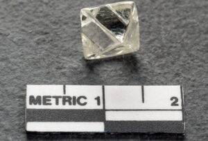
A diamond from the Colorado Wyoming kimberlites. Photo credit: Howard Coopersmith
A legacy in rocks
Dr. Lee Groat, professor in the department of Earth, Ocean and Atmospheric Sciences (EOAS), and alumna Mary Macquistan found raudseppite in barium-rich rocks in the Yukon by accident when examining samples under a microscope. They named the new mineral after late colleague Dr. Mati Raudsepp, who ran the Electron Microbeam lab. “He was quite a character—we all have Mati stories,” said Dr. Groat, who also has a mineral, groatite, named after him.
Kopylovite was discovered locked inside a ‘deep diamond’ formed about 150 kilometres beneath the Earth’s surface by alumnus Dr. Nester Korolev. He named the mineral after his former supervisor and EOAS professor, Dr. Maya Kopylova, and her father, Gerzen Kopylov. “I wanted it to be a family mineral,” said Dr. Kopylova. “My father was a role model for me—a physicist and poet who opposed the totalitarian regime of the Soviet Union.”
A rare find
About 100 minerals are discovered annually, with only 6,200 in existence, and modern minerals are often smaller than a grain of dust. Scientists have to show a unique chemistry and atomic structure to confirm and name a new mineral. Less than three per cent are named after women.
Clues from the Earth
The minerals trapped inside kopylovite provide rare insights into the makeup of the Earth’s interior: rich in potassium and titanium, its presence suggests that the area where it formed contained very little water, said Dr. Kopylova. “If more water and a compound called alumina had been present, these elements would likely have been incorporated into mica, a much more common mineral.”
Note: The above post is reprinted from materials provided by University of British Columbia.
Residue of the Cretaceous-Paleogene impact. Dark clay-rich KT boundary layer in Stevn’s Klint, Denmark used in the study. Credit: Dr. Philippe Claeys.
A rare CO chondrite meteorite was the probable impacter that struck Earth 66 million years ago, wiping out 75% of Earth’s species, including nonavian dinosaurs. These findings are published in Science Advances. Researchers at the University of British Columbia (UBC), Paris, Brussels and Vienna, used advanced nickel isotope analysis of samples to narrow down the composition of the deadly Cretaceous-Paleogene meteorite.
“Carbonaceous chondrites of the Ornans class are definitely not like the typical meteors you find in museum collections,” says Dr. Philippe Claeys, who worked on the study as a visiting professor at UBC.
“A CO contains much less volatile elements—like carbon, zinc, water and particularly sulfur—than other classes of meteorites we’ve discovered so far on Earth. It doesn’t alter our theory of what caused the extinction event—but it makes it less likely that sulfur contained in the impacter was the smoking gun. The fine debris thrown into the atmosphere would have been the primary factor.”
Researchers from Institut de Physique du Globe and Université de Paris conducted high-precision nickel isotope measurements of samples collected over years from a thin layer of clay created across the globe by the impact.
“This is challenging work,” adds Claeys, a professor with Vrije Universiteit Brussel currently visiting the Pacific Center for Isotopic and Geochemical Research with Earth, Ocean and Atmospheric Sciences at UBC. “Only a minute fraction of the projectile is preserved in the planet’s KT clay layer because the entire meteorite vaporized upon impact.”
Many questions remain about the origins of the world-shattering meteorite. Potential sources include distant, debris-rich regions of the outer solar system or even the outer area of the asteroid belt near Jupiter.
A rare impacter
Carbonaceous chondrites make up only 5% of meteorites so far sampled on Earth. Carbonaceous chondrites of the Ornans class—CO chondrites—make up a tiny fraction of that group. They are some of the most primitive and untouched materials in the solar system.
“Being impacted by such a rare, distant projectile really underscores how unlucky the dinosaurs were,” says Claeys.
The Cretaceous-Paleogene impacter was roughly 10–15 kilometers or 6 miles wide. It hit at an estimated 64,000 km/h (40,000 mph), forming the massive Chicxulub crater. The impact zone is buried underneath the Yucatán Peninsula in Mexico.
Reference:
Georgy Makhatadze, The origin of Cretaceous-Palaeogene impactor revealed by nickel isotopes, Science Advances (2026). DOI: 10.1126/sciadv.aef4858.
A research team from Okayama University of Science, Tokyo City University, the Natural History Museum, Kishiwada City (Osaka Prefecture), and other institutions has identified four previously unrecognized fossil bones from a rock containing mosasaur remains collected about 30 years ago in Kishiwada City, Osaka Prefecture.
Among the discoveries is the premaxilla, the frontmost bone of the upper jaw, which has been identified in a mosasaur fossil from Japan for the first time. The fossils also exhibit anatomical features unlike those of previously known mosasaurs, raising the possibility that they represent a new species.
Mosasaurs were large marine reptiles that lived worldwide during the Late Cretaceous, approximately 98 to 66 million years ago. The fossils were originally discovered between 1990 and 1992 in Sobura, Kaizuka City, Osaka Prefecture, and have been housed at the Natural History Museum, Kishiwada City. During a recent reexamination of unprepared rock specimens, researchers recovered four fossil bones that had remained embedded in the matrix.
One of these fossils, the premaxilla, represents the first confirmed occurrence of this bone in a Japanese mosasaur specimen and constitutes one of the study’s most significant findings. At the time of the original discovery, the limited availability of comparative mosasaur specimens made it impossible to determine the fossils’ taxonomic identity. Advances in mosasaur research over the past decades, together with the accumulation of comparative specimens and anatomical data from around the world, have now enabled researchers to recognize the bone as a premaxilla.
The team also identified distinctive features in the basisphenoid, a bone located near the braincase. These include short horn-like projections extending laterally and the absence of a ventral median groove, characteristics that differ from those of previously described mosasaurs. These anatomical traits suggest that the specimen may belong to a previously unknown species.
This discovery highlights the scientific value of reexamining unprepared specimens housed in museums and research institutions. The findings also contribute to a better understanding of marine ecosystems along the northwestern Pacific during the Cretaceous Period. Further research will be conducted to determine whether the specimen indeed represents a new species.
An artist’s impression of a pliosaur. Credit: Megan Jacobs/University of Portsmouth
For more than 25 years, Liopleurodon has been one of the world’s most recognizable prehistoric marine predators. Immortalized in the BBC’s landmark Walking with Dinosaurs series as a colossal 25-meter (82-foot) marine hunter, it captured the imagination of millions and became synonymous with the giant reptiles that ruled Jurassic seas.
Now, a new study from the University of Portsmouth published in the Journal of Vertebrate Paleontology has revealed that the real Liopleurodon was smaller than the television legend suggested, while remaining one of the most formidable apex predators of its time.
Researchers reexamined every known specimen of Liopleurodon ferox, combining evidence from a near-complete skull and two exceptionally well-preserved skeletons with extensive postcranial remains. The study provides the most accurate reconstruction of the animal’s proportions to date and resolves long-standing uncertainty over its true size.
Lead researcher Edward Bartlett, from the School of the Environment and Life Sciences at the University of Portsmouth, said, “Our study is the first comprehensive reappraisal of every specimen assigned to Liopleurodon ferox. By bringing together all of the available material, we can finally provide a robust estimate of its size and body proportions. Although it was smaller than some famous reconstructions, it was still the dominant marine predator in the Jurassic Oxford Clay seas.”
A smaller predator than legend
The analysis shows that Liopleurodon ferox reached a maximum length of just over 8 meters (26 feet), substantially smaller than estimates of 18–25 meters (59–82 feet) that have circulated for decades. Those larger figures were based on isolated giant fossil fragments that cannot confidently be assigned to Liopleurodon.
The new work also demonstrates that Liopleurodon possessed an unusually large skull, making up around a quarter of its total body length. This proportion is greater than that seen in other pliosaurs from the same ecosystem, suggesting it was capable of tackling exceptionally large prey despite its revised body size.
How old finds reshape the picture
The story of Liopleurodon stretches back more than 150 years. The species was first described in the 19th century from a single large tooth discovered near Boulogne-sur-Mer in northern France by French paleontologist Henri Émile Sauvage, who named it Liopleurodon ferox, meaning the “ferocious smooth-sided tooth.”
University of Portsmouth Emeritus Professor David Martill also worked on the paper. He said: “During the late 19th and early 20th centuries, the rapid expansion of the brickmaking industry around Peterborough exposed vast quantities of Jurassic clay. Hundreds of brickworks sprang up, driven by the area’s abundant Oxford Clay, which was cheap to extract and fire.
“Because fossils could damage bricks during firing, clay workers were paid to remove them, carefully collecting everything from belemnites, or ‘thunderbolts,’ to bones. Those discoveries caught the attention of local farmer Alfred Leeds, whose remarkable fossil collections, including complete Liopleurodon skeletons and skulls, transformed our understanding of these Jurassic predators and found their way into museums across Britain, Europe and America.”
From BBC giant to fossil evidence
Despite these discoveries, Liopleurodon received relatively little scientific attention throughout much of the 20th century. Interest surged after the 1999 BBC series Walking with Dinosaurs, in which the predator was portrayed as a 25-meter (82-foot) giant in the episode Cruel Sea.
Martill, who advised the BBC production, said the size estimate reflected the best understanding at the time and a degree of informed speculation.
“We knew there were fragmentary remains of enormous pliosaurs, and at the time it seemed reasonable that Liopleurodon might have reached extraordinary sizes. Like many scientific ideas, that estimate has now been tested against much better evidence. This new study lets the fossils speak for themselves.”
Clues to pliosaur gigantism
Rather than diminishing the importance of Liopleurodon, the revised reconstruction paints a clearer picture of one of the Jurassic’s most specialized predators. The research confirms that it was the largest aquatic vertebrate in the Oxford Clay ecosystem and occupied the top of the food chain around 165 million years ago.
The new body model also has wider implications. Applying the revised proportions to other giant Jurassic pliosaurs suggests that some closely related species, including later members of the group, reached lengths of around 12 meters (39 feet). This indicates that true gigantism evolved in pliosaurs by the Middle Jurassic and that these marine reptiles dominated the world’s oceans for around 80 million years before being replaced by mosasaurs during the Late Cretaceous.
By resolving the true size of one of paleontology’s most famous predators, the study replaces decades of speculation with the most complete and scientifically robust picture of Liopleurodon ever assembled.
Reference:
Edward O. Bartlett et al, Re-evaluating body size in the Middle Jurassic pliosaur Liopleurodon ferox Sauvage, 1873, Journal of Vertebrate Paleontology (2026). DOI: 10.1080/02724634.2026.2691149
The UB BIOST3 Research Group designs a public-facing web interface to discover the Earth’s ancient geography. Credit: University of Barcelona
Calculating a fossil’s position throughout geological history is a complex process. In paleontology and other disciplines, determining a location in the past is a challenge that requires refined computational tools to process large volumes of data. Now, the BIOST3 Research Group at the University of Barcelona has designed an open-access web interface for the general public that simplifies this process and facilitates access to high-quality paleogeographic reconstructions.
This tool, the Paleocoordinates Calculator (PACA), will help overcome the technological barrier to accessing high-quality paleogeographic reconstructions.
This accessible tool for paleogeographic research and education is presented in Scientific Reports. The authors are Noa Scholz-Murcia, Alejandro Rodríguez-Mena, Víctor Madarnás-Gómez and Antonio Monleón-Getino, from the Department of Genetics, Microbiology and Statistics at the UB’s Faculty of Biology.
Open and reproducible science
The ambition to map and understand Earth’s geography has driven major technological revolutions that have enabled the current precision of cartography. Traditional tectonic reconstruction software usually requires programming skills or the use of complex programs.
PACA helps explore Earth’s ancient geography and transforms current positions into paleocoordinates using state-of-the-art plate tectonics models.
“This innovative interface removes methodological barriers: You simply upload a CSV file containing the current coordinates and the geological age of the find to obtain the exact paleocoordinates in seconds,” explains Professor Antonio Monleón-Getino, head of the BIOST3 Research Group and member of the Bioinformatics Barcelona (BIB) platform.
In line with the principles of open science, both the PACA source code and the 3D conversion scripts are publicly available on the Zenodo repository.
The tool developed by BIOST3 offers an efficient way to process large volumes of data and promotes transparency and reproducibility in the Earth sciences. Through PACA, any researcher or user, regardless of their computing background, will be able to trace locations back through geological time.
A bridge between code and 3D visualization
The mathematical core of PACA is based on the R package palaeoverse, which connects directly to the GPlates web service.
“The tool allows users to compare their data simultaneously with up to five global plate models (GPM) widely used by the scientific community: PALEOMAP, GOLONKA, MERDITH2021, TorsvikCocks2017 and MATTHEWS2016_pmag_ref,” explains Noa Scholz-Murcia, first author of the article and a member of the Biodiversity Research Institute (IRBio) at the UB.
From paleocoordinates to the interactive viewer
In addition to providing the reconstructed paleocoordinates, PACA automatically calculates variability between models. It generates metrics such as the paleolatitudinal range and the maximum geographic distance in kilometers between the predictions of the different models. This allows researchers to immediately assess the degree of tectonic uncertainty in the study area.
The interface can export optimized tables for statistical analyses and features an interactive 3D viewer developed with React and Blender. This module projects the calculated points directly onto the paleogeographic maps of the PALEOMAP Project, created by geographer Christopher Scotese and adapted to the International Chronostratigraphic Table.
Maximum precision without installation requirements
However, does replacing desktop software affect accuracy? “Absolutely not,” says the BIOST3 team, which carried out a cross-validation with 142 reconstructions distributed globally.
The results demonstrated an almost perfect mathematical equivalence with the traditional GPlates workflow: an average spatial error of less than 17 meters, an insignificantly small distance on a planetary scale; a concordance correlation coefficient (CCC) of 1.000 across all models; and no evidence of systematic biases in the automated processing.
The PACA interface was designed as part of the research project “Cretaceous Resin Interval. Abiotic and biotic causes and their paleoecological implications (CREI),” coordinated by experts Monleón-Getino and Xavier Delclòs, from the Faculty of Earth Sciences and the IRBio. The CREI project studies the massive production of resin during a Cretaceous period that allowed the formation of many fossil resin deposits known today as amber.
Reference:
Noa Scholz-Murcia et al, A user-friendly online tool for paleocoordinate calculation and 3D visualization, Scientific Reports (2026). DOI: 10.1038/s41598-026-46309-z
Bear Island in the Barents Sea which is a paleontological hotbed known for preserving ancient microfossils. Credit: Wikipedia
How life started on our own planet may not seem as sexy as finding evidence for life on Mars, or the icy moons of Europa or Enceladus. But the search for the first eukaryotes here on Earth remains as important to astrobiology as finding life on a far-flung planet. That’s in part because for ninety percent of Earth’s history, life here was microbial.
On Earth, we had origins of life over three and a half billion years ago, Ross Anderson, a paleontologist at the U.K.’s University of Oxford, told me in his office. We had cyanobacteria and oxygenic photosynthesis at least 2.3 billion years ago; then we had eukaryotes at least 1.7 billion years ago, he says.
They were followed by algae at least a billion years ago, probably even earlier. Then the animal kingdom arrived at least 570 million years ago; probably slightly earlier.
But to find the common ancestor of the plant and animal kingdom you must go back to something like 1.6 billion years ago, says Anderson.
And so-called crown eukaryotes, the earliest eukaryotes on Earth are thought to have been fundamental to the development of complex life here on Earth. In fact, Anderson unequivocably considers eukaryotes as Earth’s first complex life.
What Are Eukaryotes?
Eukaryotes have a cell nucleus where DNA is enclosed, but they also have organelles, subcellular structures in their cells, such as the mitochondrion, that allows energy-intensive lifestyles.
It’s the eukaryotes which have developed complex multicellularity and macroscopic forms; all the animals, plants and fungi that we see around the world are eukaryotic, says Anderson.
No organism older than 500 million years had shells and skeletons as they hadn’t evolved yet. As a result, paleontologists are reliant on quite unusual environmental settings where cellular remains and soft tissues can be preserved. Consequently, researchers know very little about how life was evolving across a period which makes up 90 percent of Earth’s history.
As for Anderson?
I’m interested in how we went from a planet which just had bacteria to one which had complex multicellular organisms, says Anderson. Those kinds of multicellular fossils are hard to find, so I do a lot of work on the chemistry of the rocks to find out in which settings they are preserved, he says.
One problem is that eukaryotic microfossils are subject to billions of years of degradation.
But we know that the transition from single cellular to multicellular happened multiple times on different parts of the Earth, says Anderson. We’re interested in how animals became so diverse today, he says.
Most of their diversity got set up across the Ediacaran/Cambrian transition. That’s an epoch some 540 million years ago that represented a major evolutionary step between soft bodied biota and the Cambrian explosion of life with mobility, shells and skeletons.
As for where to look for such ancient eukaryotic microfossils?
Anderson and colleagues are particularly interested in a 100sq. km area in what was a shallow sea, some 80 degrees North in a remote group of islands near Svalbard, Norway.
And just last year, in Australia researchers found some of the oldest eukaryote microfossils ever discovered, dating back some 1.75 billion years.
The sweet spot for such microfossils usually is in ancient coastal areas, where eukaryotes would have had access to rich organics and plentiful nutrients, enabling them to grow in both multicellularity and diversity.
The idea is to go to areas that are either pristine or have not been sampled to any great extent. Anderson himself specializes in looking in areas that were subject to massive clay deposits that might have helped preserve these ancient eukaryotes.
Today, you’re looking at places that are desert or Arctic, where there’s no vegetation so rocks are exposed, says Anderson.
None of which is easy. Looking for eukaryote microfossils is truly a herculean task, because they are both tiny and consist of unprotected soft tissue which has left them subject to massive degradation over billions of years.
The biggest challenge now is that we have an under sampled fossil record, says Anderson.
Are we any closer to answering the big questions about how complex life first started here?
We’ve started to figure out which are the right rocks to find early fossils and that’s starting to give us the data with which we can record the history of Earth’s earliest life, says Anderson.
The Bottom Line?
A lot of the work we’ve done on clays was motivated by finding life on other planets, says Anderson. We’d better understand how life happened here if we hope to understand the likelihood of it happening elsewhere, he says.
Representative samples of the modern fauna (left three samples) and the Paleozoic fauna (right four samples). (Image credit: Sarah Leibovitz)
A new Stanford led study has provided the strongest evidence yet for why some marine animals survived Earth’s largest mass extinction while many others disappeared forever. The findings not only explain how modern ocean ecosystems came to be, but also offer a cautionary glimpse of how today’s warming oceans could affect marine life.
Roughly 252 million years ago, the Permian-Triassic extinction event, often called the “Great Dying,” wiped out about 96% of marine species and 70% of land animals. Yet the devastation was not evenly distributed across the tree of life.
Before the extinction, ancient seafloors were dominated for about 280 million years by brachiopods, which resemble clams, along with sea lilies (crinoids) and other bottom dwelling animals. After the catastrophe, those once dominant groups were nearly eliminated. In contrast, only about half of mollusks, including clams and snails, disappeared. The survivors, along with fish and echinoderms such as starfish and sea urchins, went on to dominate Earth’s oceans, a pattern that continues today.
Published July 6 in the Proceedings of the National Academy of Sciences, the study is the first to combine biological data from both the groups devastated by the extinction and those that survived. The results point to one major difference: species whose metabolisms were less able to cope with warmer, oxygen poor water suffered the highest extinction rates.
Those harsh ocean conditions developed after massive volcanic eruptions pumped enormous amounts of carbon dioxide and methane into the atmosphere, dramatically warming the planet.
“With this study, we essentially wanted to solve the mystery of why, when you go to the beach, you collect the shells of clams and snails rather than those of brachiopods,” said lead study author Jose Andres Marquez, a former PhD student in the lab of Erik Anders Sperling at Stanford. “Our findings show that, across different organism groups, extinctions happened at much higher rates for those more vulnerable to increases in water temperature and decreases in oxygen availability.”
Ancient Extinction Offers a Modern Climate Warning
According to the researchers, the work also has important implications for the present. The environmental conditions before the Great Dying resembled the relatively cool, oxygen rich oceans that existed for millions of years before human activities began rapidly altering Earth’s climate through fossil fuel emissions.
“This study is really the final nail in the coffin for what caused the Permian-Triassic mass extinction,” said Sperling, the study’s senior author and an associate professor of Earth and planetary sciences in the Stanford Doerr School of Sustainability. “The biggest mass extinction of all time started from a world that is very similar to today in having a relatively cool, relatively well-oxygenated ocean, and then there was a giant injection of carbon dioxide into the Earth system. Understanding how Earth and Earth’s biota responded back then could inform us of what’s to come.”
Why Metabolism Determined Survival
Metabolism includes all of the chemical processes that allow living organisms to produce energy and stay alive. During the Paleozoic era, which ended with the Great Dying, many marine animals were slow moving, bottom dwelling filter feeders, including brachiopods, crinoids (sea lilies, related to starfish), and some corals and sea anemones.
The marine animals that flourished afterward were generally much more active. Fish, mobile snails, sea urchins, and bivalves such as clams, oysters, and mussels all require faster metabolisms to support movement and, in many cases, predatory lifestyles.
Compared with brachiopods, bivalves have greater energy demands because of their larger bodies and muscular “foot” that allows them to burrow and crawl.
“This is why we eat clam chowder and we don’t eat brachiopod chowder,” Sperling said. “Brachiopods have almost no meat.”
Before the extinction, brachiopods greatly outnumbered bivalves. Today, only about 400 brachiopod species remain, while an estimated 10,000 to 15,000 species of bivalves exist.
Sperling compared this dramatic ecological shift to the extinction of the non-avian dinosaurs 65 million years ago, “where mammals essentially took over and never gave up that niche to reptiles again.”
Recreating an Ancient Ocean Crisis
The research expands on a 2018 Princeton and Stanford study, which concluded that warming oceans and oxygen loss were likely responsible for the Great Dying. However, that earlier work relied largely on physiological data collected from modern marine species, particularly economically important fish and crustaceans, leaving major gaps in knowledge about the animals that were actually hardest hit.
“In our new study, we filled in this gap about the physiology of the Paleozoic fauna to see if we could explain not only the biogeography of the extinction but the taxonomic selectivity of the extinction,” said Sperling.
To close that gap, the team conducted years of fieldwork, including collecting living brachiopods in Washington state’s San Juan Islands, where they remain relatively common. Researchers assembled a wide range of marine animals representing both ancient and modern ocean ecosystems.
At field stations and in Stanford laboratories, the scientists measured how much oxygen each organism consumed under different water temperatures. As water warms, metabolic activity speeds up, increasing an animal’s demand for oxygen.
The experiments revealed that Paleozoic animals could survive in lower oxygen conditions than many modern species. However, once temperatures rose, their slow metabolisms could no longer keep up. Their oxygen demands increased much faster than those of modern marine animals.
According to the researchers, differences in body structure help explain the result. More active modern species require more oxygen under normal conditions, but they also possess the muscles and gills needed to handle rising oxygen demands during warming.
“Warming and oxygen loss are the key drivers,” said Sperling.
Other studies have also identified ocean acidification, caused by carbon dioxide making seawater more acidic, as another stressor because it makes shell formation more difficult. Sperling said the new findings suggest acidification likely contributed to the extinction but was far less significant than warming and oxygen depletion.
Lessons for Today’s Oceans
The Stanford team plans to expand its research to additional groups of marine animals to better understand how warming, oxygen loss, and acidification interact, particularly as all three are becoming more severe in today’s oceans.
The researchers warn that history could repeat itself if modern marine species face increasingly warm, oxygen depleted waters.
“The bad news is, we are on track for Permian-Triassic levels of warming in worst-case scenario projections,” said Sperling. Temperatures increased 8-12° Celsius over thousands of years to cause the Great Dying, and today, over just 100-200 years, temperatures are projected to be 1.5-4° Celsius warmer than pre-industrial times by 2100. “But the good news is, we’re still at the point where we can change things and do something about it.”
Funding was provided by the U.S. National Science Foundation, NASA, the Palaeontological Association, and the Stanford Woods Institute for the Environment.
Reference:
J. Andres Marquez, Justin L. Penn, Richard G. Stockey, Thomas H. Boag, Murray I. Duncan, Kyra N. McClure, Kendall Matsumoto, Kemi F. Ashing-Giwa, Christopher P. Noll, Curtis Deutsch, Jonathan L. Payne, Erik A. Sperling. Differences in physiological tolerance to global warming caused the Permian–Triassic transition between the Paleozoic and Modern faunas. Proceedings of the National Academy of Sciences, 2026; 123 (28) DOI: 10.1073/pnas.2533086123
Researchers have uncovered a hidden feature beneath the Pacific Ocean that helps explain why Japan’s devastating 2011 earthquake and tsunami became so destructive. The discovery also offers new clues that could improve forecasts of future megaquakes and tsunamis.
A new study found that a thin layer of soft, clay-rich sediment beneath the Japan Trench played a critical role in the disaster. Located just below the seafloor, this unusually weak layer allowed the fault to rupture all the way to the trench during the 2011 “megathrust” earthquake. As a result, the seafloor shifted by an extraordinary 130 to 200 feet, helping generate the massive tsunami.
“That’s equivalent to the entire area between Los Angeles and San Francisco moving 130 to 200 feet in just six minutes,” said Christine Regalla, an associate professor in Northern Arizona University’s School of Earth and Sustainability and a co-author of the study. “We’ve never seen anything like that in the time we’ve been observing earthquakes. Based on what we understood, we didn’t think that could happen.”
The research, led by Regalla and more than a dozen scientists from around the world, was published in Science.
Hidden Clay Layer Beneath the Japan Trench
Most large earthquakes begin much deeper below Earth’s surface. Regalla explained that when tectonic plates shift, the rupture that produces an earthquake usually occurs far underground. For example, the rupture that caused the 6.8 magnitude Nisqually earthquake in the Pacific Northwest in 2001 started about 32 miles beneath the seafloor.
The 2011 Japan earthquake was very different. The rupture reached only about 15 miles below the seafloor, allowing the fault to break much closer to the ocean bottom. The resulting magnitude 9.1 earthquake triggered one of the deadliest natural disasters in modern Japanese history, killing nearly 20,000 people and causing more than $200 billion in damage.
To understand why this happened, researchers traveled to the western Pacific aboard the research vessel Chikyu. They drilled about 26,000 feet into the ocean floor, recovered sediment samples, and analyzed the material. Guinness World Records recognized the expedition as the deepest scientific ocean drilling project ever completed.
The samples revealed a 100 foot thick layer of pelagic clay, an extremely soft, slippery sediment formed over millions of years as microscopic particles slowly settled to the seafloor. Sandwiched between much stronger rock layers, the clay acted like a natural “tear line” that concentrated the rupture along a narrow path.
“At the Japan Trench, the geologic layering basically predetermines where the fault will form,” said study co-author Patrick Fulton, an associate professor in Cornell University’s Department of Earth and Atmospheric Sciences. “It becomes an extremely focused, extremely weak surface, which makes it easier for ruptures to propagate all the way to the seafloor.”
Why the Discovery Matters
Because this pelagic clay layer stretches for hundreds of miles along the Japan Trench, researchers believe the region may be more vulnerable to shallow slip earthquakes than previously thought. Regalla said understanding where these weak layers exist could improve scientists’ ability to identify areas capable of producing the largest earthquakes and tsunamis.
“An earthquake and tsunami in Japan doesn’t just impact people who live locally — it also impacts people at the ports and people who live across the ocean,” Regalla said. “Think about Hawaii: Their most devastating tsunamis come from Japan and Alaska. These are truly global events.”
Improving Earthquake and Tsunami Forecasts
The researchers hope the findings will help scientists better understand where powerful earthquakes and tsunamis are most likely to occur. That knowledge could help policymakers strengthen building codes, improve earthquake resistant infrastructure, update evacuation plans, and better prepare communities for future disasters.
“Japan is one of the world leaders in earthquake and tsunami preparation, but even they weren’t prepared for what happened in 2011,” Regalla said. “We all need to gain a better understanding of where these events might happen in the future. Only then can we make emergency plans that will keep everyone safe.”
Reference:
J. D. Kirkpatrick, H. M. Savage, C. Regalla, S. Shreedharan, C. Ross, H. Okuda, U. Nicholson, K. Ujiie, R. Hackney, M. Conin, P. Pei, S. Satolli, J. Zhang, P. Fulton, M. Ikari, S. Kodaira, L. Maeda, N. Okutsu, S. Toczko, N. Eguchi, P. Bellanova, C. Brown, M. Brunet, M. R. Castillo, Y.-C. Chang, M.-L. Doan, J. Everard, A. Fintel, J. Ford, R. Fukuchi, A. Gough, H. Guo, D. Gürer, M. Hagino, Y. Hamada, H. Hosono, M.J. Jurado, A. Ijiri, T. Ishikawa, M. Iwai, T. Jeppson, N. Kamiya, T. Kanamatsu, A. LaPlante, W. Lin, A. Miyakawa, Y. Morono, Y. Nakamura, C. Pizer, T. Rasbury, R. Robertson, K. Schaible, H. Sone, C. Sun, T. Uchida, P. Vannucchi, A. Yamaguchi, Y. Yamamoto, T. Yoshimoto. Extreme plate boundary localization promotes shallow earthquake slip at the Japan Trench. Science, 2026; 391 (6784): 489 DOI: 10.1126/science.ady0234
Fault-controlled basins and interpreted structural frame in the newly identified EAFBP. Credit: Nature Geoscience (2026). DOI: 10.1038/s41561-026-01991-6
Researchers have identified a massive hidden geological feature beneath the East Antarctic Ice Sheet, revealing a previously unrecognized connection between some of the continent’s largest buried landscapes.
The newly recognized structure consists of a network of enormous basins concealed beneath ice that exceeds three kilometers (nearly two miles) in thickness in some locations.
Together, these basins form a continent-scale fan-shaped pattern that researchers have named the East Antarctic Fan-shaped Basin Province.
The province encompasses several well-known subglacial features, including the Wilkes and Aurora basins, as well as the basin containing Lake Vostok, the largest known subglacial lake on Earth.
Although scientists have studied many of these basins individually for years, this is the first time they have been recognized as parts of a single, interconnected geological structure.
Evidence of Ancient Crustal Stretching
According to the research team, the structure likely formed through a process known as distributed rotational extension.
This occurs when continental crust gradually stretches outward from a central point. Researchers compare the pattern to a hand, where the base of the thumb remains fixed while the fingers spread apart. The spaces between the fingers resemble the triangular basins created as the crust extends.
The East Antarctic Fan-shaped Basin Province may represent one of the largest examples of rotational extension ever identified within continental crust.
Scientists believe the structure developed through multiple tectonic episodes associated with the formation and evolution of the ancient Gondwana supercontinent. It may also be linked to the later separation of Antarctica and Australia and could even have played a role in that continental breakup.
The discovery raises several new questions, including when the structure formed and what geodynamic processes were responsible for creating it.
Implications for Antarctica’s Ice Sheet
The importance of the finding extends beyond reconstructing Antarctica’s geological past.
The shape of the bedrock beneath the ice continues to influence how ice moves across the continent today. This hidden landscape helps determine the location of subglacial basins and lakes and may affect the stability of regions of the Antarctic Ice Sheet that are particularly vulnerable to climate change.
Mapping Antarctica’s Hidden Landscape
To investigate the newly recognized structure, researchers combined multiple sources of data, including subglacial topography, geological observations, gravity measurements, magnetic data, seismic information, and models of the crust and lithosphere.
Their analysis indicates that the feature is the result of deep tectonic processes operating within the Antarctic lithosphere.
Dr. Guy Paxman from the Department of Geography was a member of the international research team.
He led calculations estimating how East Antarctica’s landscape would appear if the entire ice sheet were removed (which would cause the land to rebound upwards by as much as one kilometer).
This reconstructed “rebounded topography” allowed researchers to examine both the elevation and orientation of the newly identified geological structure.
The study was led by Dr. Egidio Armadillo of the University of Genoa and was supported by the Italian National Antarctic Research Program.
Reference:
Egidio Armadillo, Daniele Rizzello, Pietro Balbi, Alessandro Ghirotto, Davide Scafidi, Guy J. G. Paxman, Andrea Zunino, Fausto Ferraccioli, Laura Crispini, Andreas Läufer, Frank Lisker, Antonia Ruppel, Danilo Morelli, Martin Siegert. A fan-shaped subglacial basin province in East Antarctica formed by rotational extension. Nature Geoscience, 2026; DOI: 10.1038/s41561-026-01991-6
Nearly half a century ago, a small earthquake beneath northern Utah left seismologists puzzled. The event seemed to originate far deeper than earthquakes were thought capable of occurring beneath a continent. Now, new research from the University of Utah has confirmed that the unusual quake was real and part of a rare category of seismic events happening deep within Earth’s mantle.
The earthquake struck in the early morning of February 24, 1979, beneath the town of Randolph near Utah’s borders with Idaho and Wyoming. Although it registered a magnitude of 3.8, nobody reported feeling it. The seismic recordings also appeared unusual, prompting closer examination.
At the time, University of Utah postdoctoral researcher George Zandt analyzed the data and calculated that the earthquake originated about 90 kilometers below sea level. That depth placed it well below Earth’s crust and deep within the upper mantle, a location where scientists generally did not expect earthquakes to occur.
“The deep depth explained why it wasn’t felt by people at the surface,” said Zandt, who later spent many years on the geology faculty at the University of Arizona. “I did some other analysis that convinced me of the reality of the deep depth but it was hard to convince others of the highly anomalous mantle earthquake occurring in a region where none should exist.”
Decades Later, Old Data Reveals a Pattern
Zandt published a brief abstract about the Randolph earthquake in Earthquake Notes, but the finding attracted little attention. Interest was revived decades later when University of Utah researchers revisited the original seismic records.
Led by geology professor Keith Koper, the team reexamined waveform data from the 1979 earthquake along with eight other suspected deep earthquakes that had occurred in northern Utah and southwestern Wyoming.
Their analysis confirmed that all nine events originated well below the crust, providing strong evidence for the existence of what scientists call continental mantle earthquakes (CMEs).
The findings gained additional significance when another deep earthquake struck on September 10, 2025, near Maeser in Utah’s Uinta Basin. That event reached magnitude 4.1 and originated about 68 kilometers below the surface.
Its source was located more than 20 kilometers beneath the Mohorovičić discontinuity, commonly called the Moho, which marks the boundary between Earth’s crust and the underlying mantle. In a separate study published in The Seismic Record, researchers described the Maeser earthquake as an “archetypal continental mantle event.”
Earthquakes in an Unusual Environment
Unlike most earthquakes, these deep events occur in an environment characterized by extreme heat and pressure. At such depths, rocks are generally expected to deform slowly rather than fracture suddenly.
“This is an example of an earthquake that’s nucleating in very unusual conditions, the high temperature, the high pressure, and almost all the material at that depth is going to flow. It’s more like taffy, it’s taffy on long time scales, like millions of years,” said Koper, who directs the University of Utah Seismograph Stations and once studied under Zandt. “Nevertheless, you can still see it in rocks that have made their way back up to the surface, you can see how they were stretched.”
Zandt came out of retirement to collaborate on the new research and is listed as a coauthor.
A Different Kind of Earthquake
To determine where earthquakes begin, seismologists examine the travel times of different seismic waves recorded by instruments at the surface. Small differences in arrival times help researchers pinpoint the earthquake’s origin.
The University of Utah Seismograph Stations has preserved decades of seismic records, creating a valuable archive for modern analysis. Graduate student Sean Hutchings used this archive to study known deep earthquakes and identify additional events that had previously been classified as crustal earthquakes.
“It’s sort of a mystery in terms of fundamental physics. How in the world can these things happen?” Koper said. “Another reason why it’s a big deal is that we have no idea how big they can be. With crustal earthquakes, we can measure what we think their maximum size is going to be. We measure the faults that we can map out near the surface. We can measure the length of a fault segment and that clues us into how big it can be, which helps us estimate seismic hazard.”
The researchers found several characteristics that set these deep earthquakes apart from more familiar seismic events. They occur alone, without the foreshocks and aftershocks commonly associated with shallow earthquakes. They are also concentrated near the western edge of the Wyoming Craton and occur in regions where temperatures often exceed 700 degrees Celsius.
The Role of the Wyoming Craton
The Wyoming Craton is an ancient, stable block of Earth’s lithosphere that extends beneath parts of Wyoming and neighboring states. Koper compares cratons to icebergs. Rather than floating in the ocean, they extend downward into Earth’s mantle like the keel of a ship.
Situated between the tectonically active western United States and the more stable interior of the North American plate, the Wyoming Craton has experienced significant erosion over geologic time. As a result, its structure varies across the region, and the lithosphere becomes progressively thinner toward Idaho and Utah.
The newly confirmed deep earthquakes occur in this transition zone.
“On the scale of millions of years, the mantle is hitting the craton and then flowing around it,” Koper said. “It’s that interaction where that mantle flow is being diverted around this hard cratonic root that’s causing the increased strain rate, the increased deformation and it’s also creating extra stresses. We think it’s that interaction between the keel of the iceberg and the medium around it that’s leading to these earthquakes.”
The research was published April 10 in The Seismic Record under the title “The 10 September 2025 4.1 Earthquake in Northeastern Utah, United States: An Archetypal Continental Mantle Event” and May 5, 2025, in Geophysical Research Letters under the title “Upper Mantle Earthquakes Along the Edge of the Wyoming Craton.”
Additional coauthors include Sean J. Hutchings, Fan-Chi Lin, Qicheng Zeng, Relu Burlacu, Katherine Whidden, and Valerie Springer from the University of Utah Department of Geology & Geophysics. Funding for the work was provided by the State of Utah, the U.S. Department of Energy, and the U.S. Geological Survey.
References:
Keith D. Koper, Sean J. Hutchings, Relu Burlacu, Katherine Whidden, Valerie Springer, Rigobert Tibi, Guanning Pang. The 10 September 2025 Mw 4.1 Earthquake in Northeastern Utah, United States: An Archetypal Continental Mantle Event. The Seismic Record, 2026; 6 (2): 167 DOI: 10.1785/0320260006
Sean J. Hutchings, Keith D. Koper, Relu Burlacu, Qicheng Zeng, Fan‐Chi Lin, George Zandt. Upper Mantle Earthquakes Along the Edge of the Wyoming Craton. Geophysical Research Letters, 2025; 52 (9) DOI: 10.1029/2024GL114073
Note: The above post is reprinted from materials provided by University of Utah
Antarctic ice sheet response to climate and sea level. Ross Sea ice-shelf transect for low-CO₂ conditions, corresponding to high sensitivity to forcings: (left) climate contribution, (middle) sea-level contribution, and (right) combined impacts of climate and sea-level changes.
A new study published in Nature Geoscience suggests Antarctica’s ice sheet underwent a dramatic change about one million years ago, becoming much more responsive to shifts in Earth’s climate.
The research, led by scientists at the IBS Center for Climate Physics (ICCP) at Pusan National University in South Korea, offers fresh insight into how massive ice sheets react to long term climate changes and what that could mean for future sea level rise.
Today, Antarctica contains the largest mass of ice on the planet and plays a major role in regulating global sea levels. Around one million years ago, Earth experienced a major climate transition in which ice ages became longer, colder, and more intense. Scientists refer to this period as the Mid-Pleistocene Transition. Although researchers have known about this shift for decades, exactly how Antarctica’s ice sheet responded has remained uncertain.
Simulating 3 Million Years of Climate History
One of the biggest obstacles has been the lack of realistic long term climate records needed to test ice sheet behavior under ancient conditions.
To solve this problem, the team used an advanced paleoclimate simulation recently developed at the ICCP that reconstructs global climate patterns over the past 3 million years. The simulation provided detailed temperature and precipitation data, which researchers fed into the Penn State University ice-sheet-ice-shelf model.
That model tracks changes in ice sheet movement, thickness, temperature, and elevation across Antarctica and the Northern Hemisphere. It also simulates the behavior of floating ice shelves, including those in the Ross and Weddell Seas.
Using one of South Korea’s most powerful supercomputers dedicated to basic science research, the team produced a physically consistent picture of how Earth’s major ice sheets evolved as climate conditions changed over time.
Antarctic Ice Reached a Critical Threshold
The simulations revealed that Antarctica entered an entirely different mode of behavior after the Mid-Pleistocene Transition.
Researchers identified a key atmospheric carbon dioxide threshold of roughly 240 parts per million. Once CO2 levels dropped below that point, Antarctic ice volume began responding much more dramatically to changes in atmospheric and ocean temperatures.
“After this transition, the Antarctic ice sheet reacts much more strongly to changes in climate forcing. This indicates that the system does not evolve gradually but instead becomes more responsive after crossing a particular threshold in the climate system,” said Dr. Kyung-Sook Yun, researcher at the IBS Center for Climate Physics and lead author of the study.
Why Antarctica’s Ice Expanded So Rapidly
According to the simulations, several processes worked together to accelerate Antarctic ice growth after the climate transition around one million years ago.
First, colder ocean temperatures during ice ages reduced melting beneath portions of the Antarctic ice sheet that extend below sea level. At the same time, global sea levels were approximately 50-100 meters lower than today. Lower sea levels reduced pressure on the bedrock beneath Antarctic ice shelves, allowing the land underneath to slowly rise upward. That uplift helped support additional thickening of coastal ice.
Together, these mechanisms helped create the larger and more persistent Antarctic ice sheets that later defined Earth’s ice age cycles.
“Our findings suggest that the Antarctic ice sheet was more sensitive to external forcings than previously assumed. This also raises important questions about its future response to global warming,” said Prof. Axel Timmermann, Director of the IBS Center for Climate Physics and co-author of the study.
What the Findings Could Mean for the Future
The study highlights that ice sheets may not always respond to climate change in a slow, predictable way. Instead, they can suddenly shift into a much more sensitive state after crossing critical climate thresholds.
Scientists say understanding these abrupt transitions is essential for improving future projections of Antarctic ice loss and global sea level rise.
Reference:
Kyung-Sook Yun, Axel Timmermann. Increased sensitivity of the Antarctic Ice Sheet to decreasing CO2 across the Mid-Pleistocene Transition. Nature Geoscience, 2026; DOI: 10.1038/s41561-026-01979-2