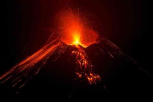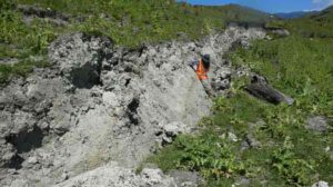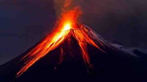

Relationship between volcanic eruptions and global monsoon hydroclimate. The bottom panel shows the distribution of global monsoon regions. Credit: Zuo Meng/Google images
Volcanic eruptions eject sulfur dioxide gas high into the atmosphere, forming sulfate aerosol chemically, and block the incoming sunlight like an umbrella. This causes surface cooling globally, but the response of global monsoon rainfall is different following volcano eruptions at different latitudes, according to quantitative research by Meng Zuo, a doctoral student from the Institute of Atmospheric Physics, Chinese Academy of Sciences, along with her mentors Prof. Tianjun Zhou and associate Prof. Wenmin Man.
This work is recently published in Journal of Climate.
Monsoon rainfall and volcano eruption
Monsoon rainfall greatly impacts society since it affects over two-thirds of the world’s population. Insufficient monsoon rainfall brings drought and famines to many parts of the world, while too much rainfall causes floods.
Following tropical volcanic eruptions, the monsoon circulation weakens and rainfall decreases consequently. But when we take the latitude of eruptions into consideration, the monsoon rainfall response changes accordingly. This phenomenon has been found in previous studies but the physical mechanism still remains inconclusive. Also the knowledge of the monsoon rainfall response to volcanic eruptions is crucial for adaptation.
The dominant role of atmospheric circulation change
The researchers analyzed large sets of data and the climate model simulations to investigate the different impacts of northern, tropical and southern volcanic eruptions on the global monsoon rainfall. “In contrast to previous work, we used a diagnostic method to quantitatively analyze the factors determining rainfall response, which is helpful to understand the different physical processes of volcanoes at different latitudes affecting the monsoon rainfall,” said Zuo.
The team found that both the proxy and observations show that monsoon rainfall in one hemisphere is reduced by the volcanic eruptions in the same hemisphere, but is enhanced by the volcanic forcing in the other hemisphere. A similar relationship is found in the model simulations.
They further advanced the underlying mechanism by using moisture budget analysis and moisture static energy budget analysis, which can decompose rainfall changes into water vapor change and circulation change. The change in atmospheric circulation is found to play a dominant role in rainfall responses. The dry-wet changes are attributed to weakened monsoon circulation and enhanced hemispheric thermal contrast, respectively. They also found that the response of the extreme rainfall is consistent with that of the mean rainfall, but more sensitive over monsoon regions, which are related to drought and flood hazards.
“This work implies that future volcanic eruptions located in different latitudes will impact the monsoon rainfall differently through circulation changes, which implies that the rainfall response to volcanic eruptions at different hemispheres should be considered in the design of Decadal Climate Prediction Project (DCPP) experiments and the implementation of geoengineering activities,” the corresponding author Tianjun Zhou, highlighted.
Reference:
Meng Zuo et al, Hydroclimate Responses over Global Monsoon Regions Following Volcanic Eruptions at Different Latitudes, Journal of Climate (2019). DOI: 10.1175/JCLI-D-18-0707.1
Many of the opals mined in Ethiopia are hydrophane opals, particularly from the Welo rocks.
Hydrophane Opal is a fresh word designed to define a specific Opal form. Opals have been mined for thousands of years in Europe and more than 165 years in Australia. However, the finding of opals from Ethiopia and Hydrophane has been around for only about 20 years. The business amounts of this product have increased over the past 10 years.
Ethiopian opal is one of today’s most varied and spectacular opal types on the market. Because this type of opal is new, there is no industry-accepted way of grading this type of opal like the black opal. Black opal is in darkness, color brightness and pattern grading.
Likewise, Ethiopian opal is also graded on shape and brightness, but the stone’s body color does not play an enormous part in determining the ultimate quality.
Ethiopian Opals have many distinctive models and the descriptions must be precise on Opal Auctions. A naturally shaped potch row with internet inclusions recognized as honey comb motif is one of the most common motifs in Ethiopian opals. In any other sort of opals, this model is very uncommon. These forms of the honeycomb are also considered to have lighter or distinct colors on occasions than the adjacent opal, which is also a unusual event in nature.
Color And Brightness In Ethiopian Welo Opal
This relates to the opal flame. These Ethiopian opals ‘ transparent inner flame has characteristics that create the flame feel 3D. In most opals, this 3-dimensional color element is uncommon. It appears to have caught flames within the opal.
Where Can You Find Welo Opal?
Ethiopia
The first released Ethiopian gem study with the finding of valuable opal in the district of Menz Gishe, North Shewa Province, was released in 1994. The opal, found mainly in the shape of nodules, was of volcanic origin and was discovered mainly in weathered rhyolite strata.
This opal Shewa Province was mostly colored dark brown and tended to break. These characteristics rendered the jewel trade unpopular. In 2008, a new opal deposit was found about 180 km north of the province of Shewa, near the town of Wegel Tena, in the Wollo province of Ethiopia. Opal from the past Ethiopian opal findings, the Wollo Province was distinct in that it more strongly resembled Australia and Brazil’s sedimentary opals with a light backdrop and often lively play-of-colour. Opal Wollo Province, more frequently referred to as opal “Welo” or “Wello,” has become the dominant Ethiopian opal in jewelry trade.
Are Ethiopian opals valuable?
Opals with a rare or unique pattern are more precious. The Harlequin pattern in opals is the most rare and loved pattern, but it is very rare.
Ethiopian opal is one of today’s market’s most varied and dramatic opal kinds. Ethiopian opal is also graded on shape and luminosity, but the stone’s body tone does not play a major part in determining the ultimate quality.
Aquilarhinus palimentus, or ‘shovel-chinned eagle nose’. Illustration by ICRA Art
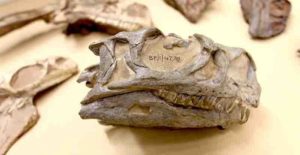
The most complete skull of a duck-billed dinosaur from Big Bend National Park, Texas, is revealed in the Journal of Systematic Palaeontology as a new genus and species, Aquilarhinus palimentus. This dinosaur has been named for its aquiline nose and wide lower jaw, shaped like two trowels laid side by side.
In the 1980s, Texas Tech University Professor Tom Lehman (then a Master’s student) was conducting research on rock layers at Rattle Snake Mountain and discovered badly-weathered bones. He and two others from the University of Texas at Austin collected them, but some were stuck together making them impossible to study. Research in the 1990s revealed an arched nasal crest thought to be distinctive of the hadrosaurid Gryposaurus. At the same time, the peculiar lower jaw was recognized. However, the specimen spent additional years waiting for a full description and it was not until recent analysis that the researchers came to realize that the specimen was more primitive than Gryposaurus and the two major groups of duck-billed dinosaurs.
“This new animal is one of the more primitive hadrosaurids known and can therefore help us to understand how and why the ornamentation on their heads evolved, as well as where the group initially evolved and migrated from,” says lead author Dr Albert Prieto-Márquez from the Institut Català de Paleontologia Miquel Crusafont, near Barcelona. “Its existence adds another piece of evidence to the growing hypothesis, still up in the air, that the group began in the southeastern area of the US.”
Duck-billed dinosaurs, also known as hadrosaurids, were the most common herbivorous dinosaurs at the end of the Mesozoic Era, and all had a similar-looking snout. The front of the jaws meet in a U-shape to support a cupped beak used for cropping plants. The beak of some species is broader than in others, but there was no evidence of a significantly different shape and therefore likely also different feeding style in duckbills until Aquilarhinus was discovered. The lower jaws of Aquilarhinus meet in a peculiar W-shape, creating a wide, flattened scoop.
Around 80 million years ago, this particular dinosaur would have been shovelling through loose, wet sediment to scoop loosely-rooted aquatic plants from the tidal marshes of an ancient delta, where today lies the Chihuahuan desert. When the dinosaur died, some of its bones were transported downstream by the tide and became lodged in vegetation. The twice-daily flow of the tide dropped silt that built up the bank of the channel around its body, fossilising the bones in thick ironstone.
The jaw and other characteristics of the specimen show that it does not fit with the main group of duck-billed dinosaurs known as Saurolophidae. It is more primitive than this group, suggesting there might have been a greater number of lineages than previously recognised that evolved before the great radiation that gave rise to the bewildering array of unadorned, solid and hollow-crested forms. Most saurolophids had bony cranial crests of many different shapes and sizes. Aquilarhinus also sported a bony crest, albeit a simple one shaped like a humped nose. The discovery of a solid crest outside the major radiation of hadrosaurids supports the hypothesis that all crests derived from a common ancestor that had a simple humped nose.
The study was funded by the Ramon y Cajal Program, the Ministry of Economy, Industry and Competitivity of Spain, the CERCA Program of the Generalitat de Catalunya, Texas Tech University, and the Sigma Xi National Scientific Honor Society.
The work was conducted under permit from the Science and Resource Management division of Big Bend National Park Service, as well as the Texas Vertebrate Paleontology Collections at The University of Texas at Austin, where the specimen is housed.
Reference:
Albert Prieto-Márquez, Jonathan R. Wagner, Thomas Lehman. An unusual ‘shovel-billed’ dinosaur with trophic specializations from the early Campanian of Trans-Pecos Texas, and the ancestral hadrosaurian crest. Journal of Systematic Palaeontology, 2019; 1 DOI: 10.1080/14772019.2019.1625078
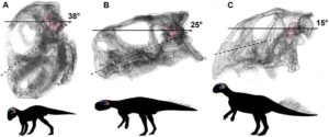
An artist’s rendering of Auroraceratops shows its bipedal posture as well as the beak and frill that characterize it as a member of the horned dinosaurs. Paleontologists from Penn led a team in characterizing this species, discovered in China. (Illustration: Robert Walters)
Many dinosaur species are known from scant remains, with some estimates suggesting 75% are known from five or fewer individuals. Auroraceratops rugosus was typical in this regard when it was named in 2005 based upon a single skull from the Gobi Desert in northwestern China. But that is no longer the case.
In the intervening years, scientists have recovered fossils from more than 80 individual Auroraceratops, bringing this small-bodied plant-eater into the ranks of the most completely known dinosaurs. It is now one of the few very early horned dinosaurs known from complete skeletons. In a collection of articles appearing as Memoir 18 in the Journal of Vertebrate Paleontology this week, researchers from the University of Pennsylvania, Indiana University of Pennsylvania, the Chinese Academy of Sciences, Gansu Agricultural University, and other institutions describe the anatomy, age, preservation, and evolution of this large collection of Auroraceratops.
Their analysis places Auroraceratops, which lived roughly 115 million years ago, as an early member of the group Ceratopsia, or horned dinosaurs, the same group to which Triceratops belongs. In contrast to Triceratops, Auroraceratops is small, approximately 49 inches (1.25 meters) in length and 17 inches (44 cm) tall, weighing on average 34 pounds (15.5 kilograms). While Auroraceratops has a short frill and beak that characterize it as a horned dinosaur, it lacks the “true” horns and extensive cranial ornamentation of Triceratops.
“When I first saw this animal back in 2004, I knew instantly it was a new kind that had never been seen before and was very excited about it,” says paleontologist Peter Dodson, senior author on the work and a professor with appointments in Penn’s School of Veterinary Medicine and School of Arts and Sciences. “This monograph on Auroraceratops is long-awaited.”
In 2005, Dodson and his former students Hai-Lu You and Matthew Lamanna named Auroraceratops (in Latin, “dawn’s horned face”) in honor of Dodson’s wife, Dawn Dodson. You, along with fellow Chinese scientist Da-Qing Li — both authors on the current work — and collaborators followed up on the discovery, identifying more than 80 additional examples of the species, from near-hatchlings to adults.
Eric Morschhauser, lead author who is now on the faculty at Indiana University of Pennsylvania, completed his Ph.D. under Dodson at Penn, focused on characterizing Auroraceratops using this robust dataset.
Auroraceratops represents the only horned dinosaur in the group Neoceratopsia (the lineage leading to and including the large bodied ceratopsians such as Triceratops) from the Early Cretaceous with a complete skeleton. This exclusiveness is significant, the researchers say, because horned dinosaurs transitioned from being bipedal, like their ancestors, to being the large rhinoceros-like quadrupedal animals most people think of as horned dinosaurs during the later parts of the Cretaceous.
“Before this study,” says Morschhauser, “we had to rely on Psittacosaurus, a more distantly related and unusual ceratopsian, for our picture of what the last bipedal ceratopsian looked like.”
Auroraceratops preserves multiple features of the skeleton, like a curved femur and long, thin claws, that are unambiguously associated with walking bipedally in some dinosaurs.
“It can now provide us with a better picture of the starting point for the changes between bipedal and quadrupedal ceratopsians,” adds Morschhauser.
Peter Dodson is a professor of anatomy in the University of Pennsylvania School of Veterinary Medicine’s Department of Biomedical Sciences and a professor of paleontology in the School of Arts and Sciences’ Department of Earth and Environmental Science.
Reference:
Hailu You, Eric M. Morschhauser, Daqing Li, Peter Dodson. Introducing the Mazongshan Dinosaur Fauna. Journal of Vertebrate Paleontology, 2019; 38 (sup1): 1 DOI: 10.1080/02724634.2017.1396995
Tamu Massif made news in 2013, thought to be the world’s largest volcano. New research offers a better look at the volcano’s formation and throws doubt on that claim.
The discovery of Tamu Massif, a gigantic volcano located about 1,000 miles east of Japan, made big news in 2013 when researchers reported it was the largest single volcano documented on earth, roughly the size of New Mexico.
New findings, reported this week in Nature Geoscience, conclude that it is a different breed of volcanic mountain than earlier thought, throwing into doubt the prior claim that it is the world’s largest single volcano.
The study analyzed magnetic field data over Tamu Massif, finding that magnetic anomalies — perturbations to the field caused by magnetic rocks in the Earth’s crust — resemble those formed at mid-ocean ridge plate boundaries.
William Sager, a geophysicist at the University of Houston and senior author for the paper, said the discovery led researchers to conclude that Tamu Massif formed by mid-ocean ridge “spreading,” the geologists’ term for creation of ocean crust at mid-ocean ridge plate boundaries, rather than as a shield volcano, as previously thought. Shield volcanos are formed primarily as stacks of fluid lava flows and are one of the most common types of volcano.
An international group of researchers — from Texas, China and Japan — sought to understand how the massive Tamu Massif volcano formed near the nexus of three spreading ridges. The key, they report, is magnetic anomalies.
Mid-ocean ridges — plate boundaries where oceanic plates move apart — are themselves large volcanoes. These ridges record distinctive linear magnetic anomalies, parallel to the ridge, as they form new crust. This is a result of lava flows and magma being concentrated near the ridge axis where the magnetic minerals in the new crust record reversals of the magnetic field polarity.
A New Understanding of Tamu Massif
Linear magnetic anomalies formed by the three ridges had previously been found around Tamu Massif, but it was unclear where they stopped within the volcano. A paper published in 2013 by Sager and colleagues concluded that Tamu Massif is an enormous shield volcano, formed by far-reaching lava flows emanating from its summit.
The latest study compiled a magnetic anomaly map over Tamu Massif, using 4.6 million magnetic field readings collected over 54 years along 72,000 kilometers of ship tracks. The data set was anchored by a new grid of magnetic profiles, positioned with modern GPS navigation, collected by the study authors using the Schmidt Ocean Institute ship Falkor. The resulting map shows that linear magnetic anomalies around Tamu Massif blend into linear anomalies over the mountain itself — implying that the underwater volcano formed by extraordinary mid-ocean ridge crustal formation.
Sager said the finding is important because it demonstrates that Tamu Massif and other oceanic plateaus are formed by a different process than previously thought. A widely-accepted model suggests a large blob of magma, known as a “mantle plume,” rises through the mantle and creates a massive volcano when it arrives at the surface. This eruption is thought to be analogous to massive eruptions on land, called “continental flood basalts” and it creates a vertical succession of lava flows.
The ocean-ridge-spreading hypothesis suggests the age progression is instead lateral. New material is always added at the center of the ridge as older material drifts laterally away. An implication is that the gradual slopes of Tamu Massif are not caused by lava flow shape but instead by a gradual inflation and then deflation of ridge volcanism as the crust became thicker and then grew thinner.
The new finding also weakens the accepted analogy between eruptions of continental flood basalts and oceanic plateaus because the formation mechanisms are shown to be different, Sager said.
‘Certainly One of the Largest’
With the discovery, Sager said Tamu Massif can no longer be considered the world’s largest shield volcano. That title reverts to Mauna Loa, on the island of Hawaii.
“The largest volcano in the world is really the mid-ocean ridge system, which stretches about 65,000 kilometers around the world, like stitches on a baseball,” Sager said. “This is really a large volcanic system, not a single volcano.”
Researchers now think Tamu Massif formed as part of that mid-ocean ridge system, he said. “Tamu Massif is certainly one of the largest volcanic mountains in the world.”
The 2013 paper was based on what researchers knew at the time, Sager said. “Science is a process and is always changing. There were aspects of that explanation that bugged me, so I proposed a new cruise and went back to collect the new magnetic data set that led to this new result.
“In science, we always have to question what we think we know and to check and double check our assumptions. In the end, it is about getting as close to the truth as possible — no matter where that leads.”
In addition to Sager, corresponding author and professor of geophysics in the UH College of Natural Sciences and Mathematics, other authors on the paper include: co-corresponding author Yanming Huang, Yangtze University; Masako Tominaga and John A. Greene, both of Texas A&M University; co-corresponding author Jinchang Zhang of the Chinese Academy of Sciences; and Masao Nakanishi of Chiba University.
Reference:
William W. Sager, Yanming Huang, Masako Tominaga, John A. Greene, Masao Nakanishi, Jinchang Zhang. Oceanic plateau formation by seafloor spreading implied by Tamu Massif magnetic anomalies. Nature Geoscience, 2019; DOI: 10.1038/s41561-019-0390-y
Along the North Anatolian Fault, Anatolia and the Eurasian Earth Plate push past each other. Image reproduced from the GEBCO world map 2014, www.gebco.net
Collapsed houses, destroyed port facilities and thousands of victims — on 22 May 1766 an earthquake of approximately 7.5 magnitude units and a subsequent water surge triggered a catastrophe in Istanbul. The origin of the quake was located along the North Anatolian fault in the Sea of Marmara. It was the last major earthquake to hit the metropolis on the Bosporus.
Researchers of the GEOMAR Helmholtz Centre for Ocean Research Kiel (Germany), together with colleagues from France and Turkey, have now been able to demonstrate for the first time with direct measurements on the seafloor that considerable tectonic strain has built up again on the North Anatolian fault below the Sea of Marmara. “It would be sufficient to trigger another earthquake with magnitudes between 7.1 to 7.4,” says geophysicist Dr. Dietrich Lange of GEOMAR. He is the lead author of the study published today in the international journal Nature Communications.
The North Anatolian fault zone marks the boundary between the Eurasian and Anatolian plates. “Strong earthquakes occur when the fault zone becomes locked. Then tectonic strain accumulates, and the seismic energy is released in an earthquake,” explains Dr. Lange. The last time this happened was in 1999 at a section of the North Anatolian fault near Izmit, about 90 kilometers east of Istanbul.
Tectonic strain build-up along fault zones on land has been regularly monitored for years using GPS or land surveying methods. This is not possible in seabed fault zones due to the low penetration depth of the GPS satellite signals under water. However, the section of the North Anatolian fault that poses the considerable threat to the Istanbul metropolitan region is located underwater in the Marmara Sea.
Up to now, it has only been possible to extrapolate, for example using land observations, whether the plate boundaries there are moving or locked. However, the methods could not distinguish between a creeping movement and the complete locking of the tectonic plates. The new GeoSEA system developed at GEOMAR measuring acoustic distances on the seabed now enables scientists for the first time to directly measure crustal deformation with mm-precision. Over a period of two and a half years, a total of ten measuring instruments were installed at a water depth of 800 metres on both sides of the fault. During this time, they carried out more than 650,000 distance measurements.
“In order to get measurements accurate within a few millimetres over several hundred of metres, very precise knowledge of the speed of sound underwater is required. Therefore, pressure and temperature fluctuations of the water must also be measured very precisely over the entire period,” explains Prof. Dr. Heidrun Kopp, GeoSEA project manager and co-author of the current study.
“Our measurements show that the fault zone in the Marmara Sea is locked and therefore tectonic strain is building up. This is the first direct proof of the strain build-up on the seabed south of Istanbul,” emphasizes Dr. Lange.
“If the accumulated strain is released during an earthquake, the fault zone would move by more than four metres. This corresponds to an earthquake with a magnitude between 7.1 and 7.4,” adds Professor Kopp. Such an event would very probably have similar far-reaching consequences for nearby Istanbul as the 1999 earthquake for Izmit with over 17,000 casualties.
Reference:
Dietrich Lange, Heidrun Kopp, Jean-Yves Royer, Pierre Henry, Ziyadin Çakir, Florian Petersen, Pierre Sakic, Valerie Ballu, Jörg Bialas, Mehmet Sinan Özeren, Semih Ergintav, Louis Géli. Interseismic strain build-up on the submarine North Anatolian Fault offshore Istanbul. Nature Communications, 2019; 10 (1) DOI: 10.1038/s41467-019-11016-z
When carbon emissions pass a critical threshold, it can trigger a spike-like reflex in the carbon cycle, in the form of severe ocean acidification that lasts for 10,000 years, according to a new MIT study.
In the brain, when neurons fire off electrical signals to their neighbors, this happens through an “all-or-none” response. The signal only happens once conditions in the cell breach a certain threshold.
Now an MIT researcher has observed a similar phenomenon in a completely different system: Earth’s carbon cycle.
Daniel Rothman, professor of geophysics and co-director of the Lorenz Center in MIT’s Department of Earth, Atmospheric and Planetary Sciences, has found that when the rate at which carbon dioxide enters the oceans pushes past a certain threshold — whether as the result of a sudden burst or a slow, steady influx — the Earth may respond with a runaway cascade of chemical feedbacks, leading to extreme ocean acidification that dramatically amplifies the effects of the original trigger.
This global reflex causes huge changes in the amount of carbon contained in the Earth’s oceans, and geologists can see evidence of these changes in layers of sediments preserved over hundreds of millions of years.
Rothman looked through these geologic records and observed that over the last 540 million years, the ocean’s store of carbon changed abruptly, then recovered, dozens of times in a fashion similar to the abrupt nature of a neuron spike. This “excitation” of the carbon cycle occurred most dramatically near the time of four of the five great mass extinctions in Earth’s history.
Scientists have attributed various triggers to these events, and they have assumed that the changes in ocean carbon that followed were proportional to the initial trigger — for instance, the smaller the trigger, the smaller the environmental fallout.
But Rothman says that’s not the case. It didn’t matter what initially caused the events; for roughly half the disruptions in his database, once they were set in motion, the rate at which carbon increased was essentially the same. Their characteristic rate is likely a property of the carbon cycle itself — not the triggers, because different triggers would operate at different rates.
What does this all have to do with our modern-day climate? Today’s oceans are absorbing carbon about an order of magnitude faster than the worst case in the geologic record — the end-Permian extinction. But humans have only been pumping carbon dioxide into the atmosphere for hundreds of years, versus the tens of thousands of years or more that it took for volcanic eruptions or other disturbances to trigger the great environmental disruptions of the past. Might the modern increase of carbon be too brief to excite a major disruption?
According to Rothman, today we are “at the precipice of excitation,” and if it occurs, the resulting spike — as evidenced through ocean acidification, species die-offs, and more — is likely to be similar to past global catastrophes.
“Once we’re over the threshold, how we got there may not matter,” says Rothman, who is publishing his results this week in the Proceedings of the National Academy of Sciences. “Once you get over it, you’re dealing with how the Earth works, and it goes on its own ride.”
A carbon feedback
In 2017, Rothman made a dire prediction: By the end of this century, the planet is likely to reach a critical threshold, based on the rapid rate at which humans are adding carbon dioxide to the atmosphere. When we cross that threshold, we are likely to set in motion a freight train of consequences, potentially culminating in the Earth’s sixth mass extinction.
Rothman has since sought to better understand this prediction, and more generally, the way in which the carbon cycle responds once it’s pushed past a critical threshold. In the new paper, he has developed a simple mathematical model to represent the carbon cycle in the Earth’s upper ocean and how it might behave when this threshold is crossed.
Scientists know that when carbon dioxide from the atmosphere dissolves in seawater, it not only makes the oceans more acidic, but it also decreases the concentration of carbonate ions. When the carbonate ion concentration falls below a threshold, shells made of calcium carbonate dissolve. Organisms that make them fare poorly in such harsh conditions.
Shells, in addition to protecting marine life, provide a “ballast effect,” weighing organisms down and enabling them to sink to the ocean floor along with detrital organic carbon, effectively removing carbon dioxide from the upper ocean. But in a world of increasing carbon dioxide, fewer calcifying organisms should mean less carbon dioxide is removed.
“It’s a positive feedback,” Rothman says. “More carbon dioxide leads to more carbon dioxide. The question from a mathematical point of view is, is such a feedback enough to render the system unstable?”
“An inexorable rise”
Rothman captured this positive feedback in his new model, which comprises two differential equations that describe interactions between the various chemical constituents in the upper ocean. He then observed how the model responded as he pumped additional carbon dioxide into the system, at different rates and amounts.
He found that no matter the rate at which he added carbon dioxide to an already stable system, the carbon cycle in the upper ocean remained stable. In response to modest perturbations, the carbon cycle would go temporarily out of whack and experience a brief period of mild ocean acidification, but it would always return to its original state rather than oscillating into a new equilibrium.
When he introduced carbon dioxide at greater rates, he found that once the levels crossed a critical threshold, the carbon cycle reacted with a cascade of positive feedbacks that magnified the original trigger, causing the entire system to spike, in the form of severe ocean acidification. The system did, eventually, return to equilibrium, after tens of thousands of years in today’s oceans — an indication that, despite a violent reaction, the carbon cycle will resume its steady state.
This pattern matches the geological record, Rothman found. The characteristic rate exhibited by half his database results from excitations above, but near, the threshold. Environmental disruptions associated with mass extinction are outliers — they represent excitations well beyond the threshold. At least three of those cases may be related to sustained massive volcanism.
“When you go past a threshold, you get a free kick from the system responding by itself,” Rothman explains. “The system is on an inexorable rise. This is what excitability is, and how a neuron works too.”
Although carbon is entering the oceans today at an unprecedented rate, it is doing so over a geologically brief time. Rothman’s model predicts that the two effects cancel: Faster rates bring us closer to the threshold, but shorter durations move us away. Insofar as the threshold is concerned, the modern world is in roughly the same place it was during longer periods of massive volcanism.
In other words, if today’s human-induced emissions cross the threshold and continue beyond it, as Rothman predicts they soon will, the consequences may be just as severe as what the Earth experienced during its previous mass extinctions.
“It’s difficult to know how things will end up given what’s happening today,” Rothman says. “But we’re probably close to a critical threshold. Any spike would reach its maximum after about 10,000 years. Hopefully that would give us time to find a solution.”
This research was supported, in part, by NASA and the National Science Foundation.
Reference:
Daniel H. Rothman. Characteristic disruptions of an excitable carbon cycle. Proceedings of the National Academy of Sciences, 2019; 201905164 DOI: 10.1073/pnas.1905164116
Polar ice caps on Mars are a combination of water ice and frozen CO2. Like its gaseous form, frozen CO2 allows sunlight to penetrate while trapping heat. In the summer, this solid-state greenhouse effect creates pockets of warming under the ice, seen here as black dots in the ice.
People have long dreamed of re-shaping the Martian climate to make it livable for humans. Carl Sagan was the first outside of the realm of science fiction to propose terraforming. In a 1971 paper, Sagan suggested that vaporizing the northern polar ice caps would “yield ~10 s g cm-2 of atmosphere over the planet, higher global temperatures through the greenhouse effect, and a greatly increased likelihood of liquid water.”
Sagan’s work inspired other researchers and futurists to take seriously the idea of terraforming. The key question was: are there enough greenhouse gases and water on Mars to increase its atmospheric pressure to Earth-like levels?
In 2018, a pair of NASA-funded researchers from the University of Colorado, Boulder and Northern Arizona University found that processing all the sources available on Mars would only increase atmospheric pressure to about 7 percent that of Earth – far short of what is needed to make the planet habitable.
Terraforming Mars, it seemed, was an unfulfillable dream.
Now, researchers from the Harvard University, NASA’s Jet Propulsion Lab, and the University of Edinburgh, have a new idea. Rather than trying to change the whole planet, what if you took a more regional approach?
The researchers suggest that regions of the Martian surface could be made habitable with a material — silica aerogel — that mimics Earth’s atmospheric greenhouse effect. Through modeling and experiments, the researchers show that a two to three-centimeter-thick shield of silica aerogel could transmit enough visible light for photosynthesis, block hazardous ultraviolet radiation, and raise temperatures underneath permanently above the melting point of water, all without the need for any internal heat source.
The paper is published in Nature Astronomy.
“This regional approach to making Mars habitable is much more achievable than global atmospheric modification,” said Robin Wordsworth, Assistant Professor of Environmental Science and Engineering at the Harvard John A. Paulson School of Engineering and Applied Sciences (SEAS) and the Department of Earth and Planetary Science. “Unlike the previous ideas to make Mars habitable, this is something that can be developed and tested systematically with materials and technology we already have.”
“Mars is the most habitable planet in our Solar System besides Earth,” said Laura Kerber, Research Scientist at NASA’s Jet Propulsion Laboratory. “But it remains a hostile world for many kinds of life. A system for creating small islands of habitability would allow us to transform Mars in a controlled and scalable way.”
The researchers were inspired by a phenomenon that already occurs on Mars.
Unlike Earth’s polar ice caps, which are made of frozen water, polar ice caps on Mars are a combination of water ice and frozen CO2. Like its gaseous form, frozen CO2 allows sunlight to penetrate while trapping heat. In the summer, this solid-state greenhouse effect creates pockets of warming under the ice.
“We started thinking about this solid-state greenhouse effect and how it could be invoked for creating habitable environments on Mars in the future,” said Wordsworth. “We started thinking about what kind of materials could minimize thermal conductivity but still transmit as much light as possible.”
The researchers landed on silica aerogel, one of the most insulating materials ever created.
Silica aerogels are 97 percent porous, meaning light moves through the material but the interconnecting nanolayers of silicon dioxide infrared radiation and greatly slow the conduction of heat. These aerogels are used in several engineering applications today, including NASA’s Mars Exploration Rovers.
“Silica aerogel is a promising material because its effect is passive,” said Kerber. “It wouldn’t require large amounts of energy or maintenance of moving parts to keep an area warm over long periods of time.”
Using modeling and experiments that mimicked the Martian surface, the researchers demonstrated that a thin layer of this material increased average temperatures of mid-latitudes on Mars to Earth-like temperatures.
“Spread across a large enough area, you wouldn’t need any other technology or physics, you would just need a layer of this stuff on the surface and underneath you would have permanent liquid water,” said Wordsworth.
This material could be used to build habitation domes or even self-contained biospheres on Mars.
“There’s a whole host of fascinating engineering questions that emerge from this,” said Wordsworth.
Next, the team aims to test the material in Mars-like climates on Earth, such as the dry valleys of Antarctica or Chile.
Wordsworth points out that any discussion about making Mars habitable for humans and Earth life also raises important philosophical and ethical questions about planetary protection.
“If you’re going to enable life on the Martian surface, are you sure that there’s not life there already? If there is, how do we navigate that,” asked Wordsworth. “The moment we decide to commit to having humans on Mars, these questions are inevitable.”
Reference:
R. Wordsworth, L. Kerber & C. Cockell. Enabling Martian habitability with silica aerogel via the solid-state greenhouse effect. Nature Astronomy, 2019 DOI: 10.1038/s41550-019-0813-0
A fresh surface rupture of the Kekerengu fault, taken 4 days after the Kaikoura earthquake, with lead author Jesse Kearse leaning next to a curved slickenline (the subject of this article). Photo credit – Professor Tim Little (Victoria University of Wellington).
Slip-parallel grooves (striations) on fault surfaces are considered a robust indicator of fault slip direction, yet their potential for recording aspects of earthquake rupture dynamics has received little attention. During the 2016 Kaikōura earthquake (South Island, New Zealand), >10 m of dextral strike-slip on the steeply dipping Kekerengu fault exhumed >200 m2 of fresh fault exposure (free faces) where it crossed bedrock canyons. Inscribed upon these surfaces, we observed individual striae up to 6 m long, all of which had formed during the earthquake. These were typically curved. Using simulations of spontaneous dynamic rupture on a vertical strike slip fault, we reproduce the curved morphology of striae on the Kekerengu fault.
Assuming strike-slip pre-stress, our models demonstrate that vertical tractions induced by slip in the so-called cohesive zone result in transient changes in slip direction. We show that slip-path convexity is sensitive to the direction of rupture propagation. To match the convexity of striae formed in 2016 requires the rupture to have propagated in a northeast direction, a prediction that matches the known rupture direction of the Kaikōura earthquake. Our study highlights the potential for fault striae to record aspects of rupture dynamics, including the rupture direction of paleo strike-slip earthquakes.
The direction of earthquake rupture propagation exerts a profound influence on the distribution of strong ground shaking. As a consequence, damage and loss experienced by a community during an earthquake is dependent on the community’s location relative to the direction of rupture propagation—a relationship especially true for large strike-slip events (Somerville et al., 1997; Gomberg et al., 2001).
This effect has been observed in many large magnitude strike-slip earthquakes in recent decades; e.g., the 1992 Mw 7.3 Landers (California) earthquake (Velasco et al., 1994), the 2002 Mw 7.9 Denali (Alaska) earthquake (Eberhart-Phillips et al., 2003), and the 2018 Mw 7.5 Palu (Indonesia) earthquake (Bao et al., 2019). Based on historical data, it is uncertain whether large magnitude earthquakes systematically repeat their rupture direction; moreover, establishing the direction of past earthquakes using geological data has proved difficult. Previous studies have used structural data such as branching fault intersections (Poliakov et al., 2002; Fliss et al., 2005) and off-fault damage patterns in both ancient fault zones (Di Toro et al., 2005) and recent surface ruptures (Klinger et al., 2018) to infer rupture direction. However, these studies lack a context of seismological data with which to verify the rupture direction during a particular event.
Based on our literature review, out of ~55 surface ruptures observed geologically in the field since the late 1800s (Wesnousky, 2008; Biasi et al., 2013), 20 of the field datasets include measurements of coseismic slickenlines. Of these, 70% are curved, indicating that coseismic changes in slip direction are common (see the GSA Data Repository1 and references therein). Spudich et al. (1998) used the curvature of slickenlines (up to 50°) found on the Nojima fault following the 1995 Kobe (Japan) earthquake to infer the magnitude of shear traction on the fault surface. However, aside from this pioneering work, the potential link between curved slickenlines and the dynamics of earthquake rupture has received little attention. In this study, we propose that striae produced on fault plane surfaces during coseismic slip can reveal aspects of the dynamic rupture process.
We present new slickenline data from fault surfaces that were exposed during the 2016 Mw 7.8 Kaikōura earthquake (South Island, New Zealand)—an event that has a well-established southwest-northeast rupture direction across ~200 km of the Pacific-Australian plate boundary in New Zealand (Hamling et al., 2017; Kaiser et al., 2017; Ando and Kaneko, 2018; Litchfield et al., 2018) (Fig. 1A). We observed curved coseismic striae on multiple fault outcrops along a 10 km section of the Kekerengu fault, the structure that yielded the greatest slip and moment release during this earthquake (Cesca et al., 2017; Holden et al., 2017). The systematic convexity of these striae records temporal changes in the coseismic slip direction on this fault. To uncover the mechanism that was responsible for the observed variation in slip direction, we undertook dynamic rupture modeling of a vertical strike-slip fault, using a simple set of boundary conditions. Here we discuss the potential for curved striae to record the rupture direction of paleo strike-slip earthquakes.
Curved Striae on the Kekerengu Fault
The Kekerengu fault is part of the Marlborough Fault System, a series of mainly dextral faults that transfer slip between the Hikurangi megathrust and the Alpine fault. Dextral offset of Pleistocene terraces and uplift of the Seaward Kaikōura Ranges on its western side show that the Kekerengu fault is primarily strike-slip, with a lesser reverse component (Van Dissen et al., 2016). During the Kaikōura earthquake, many stream canyons were dextrally displaced 8–10 m and uplifted on their northwest sides by 1–2 m across the Kekerengu fault, which dips steeply to the northwest (>65° dip) (Kearse et al., 2018). Offset of these steep canyon walls (slopes of 20–30°) exhumed more than a dozen smooth and near-planar fault surfaces that were ≤7 m long in the slip direction, each coated in a 1–2 cm layer of soft fault gouge. Nine of these free faces hosted coseismic fault striae that were curved. For example, Figure 1D depicts a striation where slip initiated as dextral-reverse motion, and as further displacement accrued, the direction of slip curved to become nearly pure strike-slip.
This convex-up slip path was repeated at six out of the nine sites that contained curved striae, with some sites containing many measurement locations where striae were recorded. Curved striae were found mostly on the upper part of the free face, suggesting they were formed early in the rupture. The angular magnitude of the observed convexity is typically ~15° and is >40° at sites 3 and 7. At two sharp bends in the fault trace, the sense of uplift was opposite to the dominant one, and their striae describe a convex-down slip path. In all cases, the incremental magnitude of fault slip—both vertical and dextral—recorded by the individual fault striae segments (0.2–6 m) amounts to only a fraction of the known coseismic net displacement at these sites, which was 8–10 m.
Post-earthquake erosion of free faces in the days to months following the earthquake undoubtedly curtailed the length of individual straie; however, some striae become increasingly diffuse toward their ‘downstream’ ends , suggesting a different process is responsible for their limited length. Near-fault geodetic and seismological data collected at two stations (the KEKS seismic station, and a high-rate continuous GPS station located 30 km northeast of the study area) on the northwest side of the Kekerengu fault during the earthquake (Fig. 2A; see the Data Repository) imply that the initial ~5 s of rupturing on the Kekerengu fault accumulated up to 4 m of almost pure dextral-slip and <0.3 m of throw, whereas most of the throw (1–2 m) began accumulating 4–7 s after this. The available geological and geophysical data suggest that the curved striae on the Kekerengu fault were inscribed during the early phase of strike-slip–dominated rupturing.
Dynamic Rupture Model
To evaluate possible mechanisms for the curvature of Kekerengu fault striae, we simulated the spontaneous, dynamic rupture of a 50-km-long and 25-km-deep vertical strike-slip fault in layered elastic half space, using a spectral-element code (Ampuero, 2002; Kaneko et al., 2008). A horizontal initial shear traction was applied to the fault surface, with a magnitude that increased linearly with depth. Dynamic rupture was initiated by overstressing a small 3-km-wide patch in the center of the fault at a depth of 12 km, and then the rupture propagated spontaneously across the fault surface, where it was governed by slip-weakening friction laws (for additional details of the model setup, see the Data Repository).
Slip paths for 42 nodes on the fault surface (gray arrows in Fig. 3C) depict cseismic motion of the near-side of the fault relative to the far side. Their lengths depict slip magnitudes, and their shape and curvature illustrates any changes in slip direction. At depths >3 km, slip paths are horizontal and show little change in slip direction with time. For nodes located along mixed-mode rupture directions (Andrews, 1994) at depths <3 km, slip paths are more complex. At depths <3 km, slip follows a curved path during the initial few decimeters; at locations between x = 0 and x = –20 km, curvature is convex-up (Fig. 3A), while on the other side of the hypocenter between x = 0 and x = 20 km (right side of Fig. 3C), curvature is convex-down. As further displacement is accrued, slip directions converge toward a horizontal rake of 180°. These results do not necessarily imply that one side of the fault experiences an opposing sense of net uplift at either end of a rupture (this is only true for cases with pure strike-slip pre-stress). Rather, our results suggest that the convexity of the initial slip path is opposite at either end of the rupture, regardless of the rake of initial shear traction on the fault.
Mechanism for Changes in Slip Direction
The mechanism behind transient changes in slip direction in our dynamic model is consistent with the one proposed by Spudich et al. (1998). Dynamic changes in rake angle are driven by vertical stress changes along mixed-mode rupture directions produced within the so-called cohesive zone (the part of the fault that is slipping but has not yet fully weakened). Seismic waves are continuously generated within this zone, and they carry vertical stresses that induce vertical components of slip on the sliding surface.
At depths below 3 km, confining stresses are large compared to the dynamic loads, a relationship that suppresses the magnitude of these transient vertical motions. Yet slip at these depths retains subtle (<2°) temporal changes in slip direction, and exhibits the same reversal in path convexity on either side of the hypocenter (left versus right sides of Figure 3C are yellow and green, respectively; see the Data Repository).
Near Earth’s surface, where confining stresses are low, the ratio of dynamic to confining stress is larger, promoting a larger magnitude of coseismic vertical slip. As the rupture front propagates along strike, the model predicts opposite senses of slip deflection near the two propagating rupture tips: convex-upward on one side and convex-downward on the other. Figure 4 details changes in shear traction and slip velocity at the rupture tip to highlight the correlation between vertical stress and rotation of the slip direction.
Discussion and Conclusions
We note a correlation between the convexity of curved striae on the Kekerengu fault and results of our dynamic rupture model. As slip initiates, movement of the downstream side of the fault (the side moving in the direction of rupture propagation) follows a convex-up slip path that initially has a rake of ~15° to (and ultimately becomes parallel with) the direction of initial shear stress on the fault (Fig. 3A). Although several of our sites—specifically those at sharp fault bends—showed the opposite sense of slip-path convexity, we suggest that the kinematic differences at these areas induced local stresses that overwhelmed the more general dynamic effects described by our model. We therefore interpret the predominant pattern of slip-path curvature on the Kekerengu fault to have resulted from vertical stress changes in the cohesive zone of the northeast-propagating rupture of the Kaikōura earthquake. In addition, the curvature of striae seen on multiple exposures of the Nojima fault following the 1995 Mw 7.2 Kobe (Japan) earthquake (Otsuki et al., 1997) is consistent with our model, and with the known direction of rupture propagation in this event (Yoshida et al., 1996). These dynamic effects are likely not to be restricted to strike-slip faults, as mixed-mode dynamic rupture on dip-slip faults should also produce transient changes in initial slip direction, which may explain curved striae seen after events such as the 1954 M 7.0 Fairview Peak (Nevada, USA) (Slemmons, 1957) and 2011 Mw 6.6 Fukushima (Japan) earthquakes (Otsubo et al., 2013).
We offer two possible explanations for why striae on the Kekerengu fault capture only an early and small (typically <10% of total) increment of the 2016 slip. One possibility is that, at the onset of slip, the fault plane (in the near surface) was rough compared to the final stages of slip, having only just broken any cohesion gained during the interseismic period. If so, this might promote asperity ploughing and striae production at that early stage (Tesei et al., 2017), thus promoting a temporal bias in the striation record. According to this scenario, the early-formed asperities (i.e., topography in the new fracture surface) were progressively abraded during the accumulating slip, resulting in a smoother fault plane and a termination in striation production. Another possibility (and one that is not mutually exclusive with the former) is that during slip in the near-surface, along-strike translation of large (meter-scale) corrugations in the fault surface (e.g., Candela et al., 2012) promoted transient separation of the fault walls, thereby terminating the engraving process. Both ideas are supported by individual striae that are deeply inset near their inception point but are shallower and more diffuse toward their termination.
Spudich et al. (1998) together with Guatteri and Spudich (1998)—both of which assume depth-independent pre stress—suggest that the fractional stress drop, defined as the ratio of the stress drop to the magnitude of initial shear stress, is ~0.7 on faults that exhibit large (>30°) changes in coseismic slip direction. In our model that features depth-dependent stress, in order to reproduce up to ~20° changes in slip direction on the Kekerengu fault, the fractional stress drop is ~0.2, which corresponds to the ‘high stress’ case of Guatteri and Spudich (1998). Even in the case of ‘low stress’, the pattern of slip-path convexity should still depend on rupture direction.
Striated fault surfaces are routinely measured in neotectonic and paleoseismic studies, including on well preserved Holocene scarps and on excavated fault surfaces in paleoseismic trenches. Crosscutting or overlapping striae seen in such places do not necessarily represent the superposition of multiple earthquakes; and our results provide a simple explanation for transient changes in slip direction during a single slip episode, which can create overlapping striae (e.g., the 2011 Fukushima earthquake; Otsubo et al., 2013). More importantly, our study demonstrates that it may be possible to infer the rupture direction of paleoearthquakes in cases where coseismic striae record temporal changes in slip direction. To do this, we propose that data be collected from structurally simple parts of the fault that are representative of its overall kinematics, and that are also likely to generate and preserve striae. We further suggest that multiple sites be evaluated to establish any systematic patterns in striation convexity.
Temporal changes in slip direction during dynamic rupture are likely to be a widespread characteristic in the near-surface during large-magnitude earthquakes. Geological evidence of this type, when combined with simulations of dynamic rupture, may yield important insight into the near-field dynamics of fault slip, including the rupture direction of paleo strike-slip earthquakes and, by inference, the rupture direction of future strike-slip earthquakes; thereby helping to better constrain the distribution of damaging ground shaking in those events.
Reference:
Jesse Kearse, Yoshihiro Kaneko, Tim Little, Russ Van Dissen; Curved slickenlines preserve direction of rupture propagation. Geology doi: https://doi.org/10.1130/G46563.1
Earthquake in Southern California. Credit: Public Domain
The odds that Southern California will experience another earthquake of magnitude 7 or greater in the next week are now nearly 11%, according to preliminary estimates from seismologists.
And the chances that a quake will surpass the 7.1 temblor that struck near Ridgecrest on Friday night are roughly 8% to 9%, said Caltech seismologist Lucy Jones.
“There’s about a 1 in 10 chance that we could have another 7 in this sequence,” she said.
More likely is that the Owens Valley will experience another temblor of magnitude 6 or greater. The odds of that are slightly greater than 50-50, Jones said. And more quakes of magnitude 5 or greater are a near certainty.
“It would be extremely unusual if we didn’t have another 5” over the coming week, Jones said.
The 7.1 quake on Friday night was about 8 times larger than the 6.4 quake on Thursday morning, said Robert Graves, a seismologist with the U.S. Geological Survey in Pasadena.
Though such quakes would be more likely to occur in the next few days, the shaking could continue for quite some time.
“A magnitude 7 usually has aftershocks that last for years,” Jones said.
Jones said she could not recall a pattern of earthquakes in California where a 6.4 foreshock was followed by a 7.1 event, only to be followed by an even bigger quake.
But that doesn’t mean it can’t happen, she cautioned.
“It is clearly a very energetic sequence, so there’s no reason to think we can’t have more large earthquakes,” she said.
The last time California experienced a quake of this size was in 1999, when the 1999 Hector Mine quake struck the Mojave Desert. There were minor injuries and no deaths.
The years since have been marked by an unusual earthquake drought.
“In California, we expect to have a magnitude 7 once every 10 to 20 years, and the last one was 20 years ago,” Jones said. “Think of this as a return to what California is supposed to be doing.”
But she also said the activity near Ridgecrest is not likely to trigger any activity on the San Andreas fault.
The 7.1 quake occurred on the same fault system as the 6.4 temblor that is now being considered a foreshock. It was further away from Los Angeles, though still in the Owens Valley.
“This happened at the end of the zone that moved previously,” Jones said.
As of 11 p.m., it has already been followed by three quakes above a magnitude 5, 17 above a magnitude 4 and more than 70 that exceeded magnitude 3, Jones said.
She said the fault is now likely to be 25 to 30 miles long.
“The fault is growing,” Jones said.
Thursday’s 6.4 foreshock triggered shaking in Ridgecrest of intensity 8. With Friday’s 7.1 main shock, the shaking intensity reached a 9, Jones said.
“My expectation is that Ridgecrest is having a pretty difficult time tonight,” Jones said.
“We don’t get the 7s very often,” she added.
Note: The above post is reprinted from materials provided by Los Angeles Times . The original article was written by Karen Kaplan .
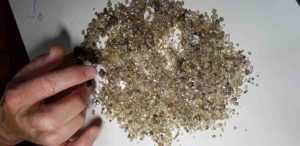
Turquoise is an opaque, blue-to-green mineral with the chemical formula CuAl6(PO4)4(OH)8·4H2O, a hydrated copper and aluminum phosphate. It is common and useful in higher grades and has been appreciated for thousands of years as a gemstone and ornamental stone due to its distinctive shade. Recently, the implementation of medicines, imitations and synthetics on the market has devalued turquoise, like most other opaque gems.
Turquoise Properties
The finest of turquoise, or slightly more than window glass, reaches a peak Mohs hardness of just under 6. A cryptocrystalline mineral characteristic, turquoise almost never creates single crystals, and all its characteristics are extremely variable. X-ray diffraction analysis proves to be triclinic in its crystal system. With reduced strength produces reduced particular pressure (2.60–2.90) and higher porosity; the grain size depends on these characteristics.
Turquoise luster is typically waxy to subvitreous, and its transparency is generally opaque, but in thin parts it may be semitranslucent. Color is as variable as the other characteristics of the mineral, varying from white to a blue powder to a purple sky, and from a green blue to a green yellow. The blue is ascribed to idiochromatic copper whereas the green may result from either iron impurities (aluminum replacement) or dehydration.
How Turquoise Is Formed?
Turquoise shapes as a secondary mineral by the activity of percolating acidic aqueous solutions during weathering and oxidation of pre-existing minerals. For instance, copper may come from main copper sulfides such as chalcopyrite or secondary carbonates malachite or azurite; aluminum may come from feldspar; and apatite phosphorus.
As turquoise is typically found in arid areas, filling or encrusting cavities and fractures in typically extremely modified volcanic rocks, often associated with limonite and other iron oxides, climatic variables appear to play an significant part. Turquoise is almost invariably combined with copper sulfide deposits weathering products in or around potassium-feldspar-bearing porphyritic intrusives in the southwestern United States.
Potassium aluminum sulfate is a prominent secondary mineral in some cases of alunite. Typically turquoise mineralization is limited to a comparatively shallow depth of less than 20 meters (66 feet), although it occurs in deeper fracture areas where secondary solutions have higher penetration or water table depth is higher.
Turquoise is almost always cryptocrystalline and huge and requires no clear internal form. Crystals are exceedingly uncommon even on a microscopic scale. Typically the shape is in habit of filling vein or fracture, nodular or botryoidal. Forms of stalactitis were recorded. Feldspar, apatite, other minerals, or even fossils can also be pseudomorphically replaced by turquoise. Odontolite is a fossil bone or ivory traditionally believed to have been changed by turquoise or similar minerals of phosphate such as iron phosphate vivianite. Also prevalent is intergrowth with other secondary minerals of copper such as chrysocolla.
Where Turquoise is found?
These are all small-scale activities, often seasonal due to the restricted deposit size and remoteness. Most of them are handmade with little or no mechanization. However, turquoise is often retrieved, particularly in the United States, as a by-product of large-scale copper mining activities.
United States
Arizona, California (San Bernardino, Imperial, Inyo counties), Colorado (Conejos, El Paso, Lake, Saguache counties), New Mexico (Eddy, Grant, Otero, Santa Fe counties) and Nevada (Clark, Elko, Esmeralda counties, Eureka, Lander, Mineral County and Nye counties) are (or were) particularly wealthy. Pre-Columbian Native Americans mined California and New Mexico’s reserves using stone tools, some local and some as far remote as southern Mexico. Cerrillos, New Mexico is believed to be the site of the earliest mines; the state was the biggest producer of the country before the 1920s; it is now more or less depleted. Today, only one mine at Apache Canyon in California works at a business capability.
The turquoise happens in the form of vein or seam fillings and as compact nuggets, most of which are tiny in number. While sometimes quite good fabric is discovered, rivaling Iranian fabric in both color and durability, most American turquoise is of small grade (called “chalk turquoise”); elevated iron levels imply predominance of greens and yellows, and a typically friendly consistency in the untreated state of the turquoise precludes jewelry use.
Currently Arizona is the most important value producer of turquoise. There are several mines in the state, two of which are renowned for their distinctive color and performance and regarded the finest in the sector: in August 2012, the Sleeping Beauty Mine in Globe stopped turquoise mining. Due to the increasing world market price of copper, the mine chose to ship all the ore to the crusher and focus on copper manufacturing. The cost of untreated natural sleeping beauty turquoise has increased dramatically since the closure of the mine. As of 2015, the Kingman Mine is still operating outside the town alongside a copper mine. Other mines include the Blue Bird mine, Castle Dome, and Ithaca Peak, but are largely inactive owing to elevated operating costs and federal laws. Bisbee’s Phelps Dodge Lavender Pit mine came to a halt in 1974 and never had a turquoise contractor. All the turquoise Bisbee was mined with “dinner pail.” It arrived in the dinner pails of miners from the copper ore mine. Morenci and Turkey Peak are either idle or exhausted.
Nevada is the other major producer of the country, with more than 120 mines producing large amounts of turquoise. Unlike elsewhere in the US, most of the Nevada mines were mainly used for their turquoise gem and very little was retrieved as a by-product of other mining activities. Nevada turquoise is discovered as nuggets, fracture fillings and interstices between pieces are discovered in breccias as the cement coating. A majority of the material produced is hard and dense because of the geology of the deposits of Nevada, being of sufficient quality that no treatment or improvement is required. Although almost every state county has yielded some turquoise, the main manufacturers are in the counties of Lander and Esmeralda. Most of Nevada’s turquoise deposits happen along a broad range of tectonic activity coinciding with the thrust fault area of the state. It strikes at a bearing of about 15 ° and stretches from the southern portion of Elko County to the south-west boundary of Tonopah in California. Nevada has created a broad variety of colors and combinations of multiple matrix motifs, with Nevada turquoise coming in distinct colors of blue, blue-green, and green. Some of this unusually colored turquoise may involve important zinc and iron, causing the lovely tones of light green to yellow-green. Some of the colors of blue to green-yellow may effectively be variscite or faustite, which is comparable in shape to turquoise secondary phosphate minerals.
Egypt
Since at least the First Dynasty (3000 BCE) in ancient Egypt, and probably before that, the Egyptians used turquoise and the Sinai Peninsula was mined by them. This area was regarded by the indigenous Monitu as the Turkey Country. The peninsula has six mines, all on its southwest shore, spanning an area of approximately 650 km2 (250 sq mi). From a historical view, the two most significant of these mines are Serabit el-Khadim and Wadi Maghareh, one of the earliest recognized mines. The former mine is about 4 kilometers from an old temple devoted to the Hathor deity.
The turquoise is discovered in basalt-covered sandstone, or was initially overlain. There are works of copper and iron in the region. Large-scale turquoise mining is not lucrative today, but Bedouin populations use homemade weapons to quarry the deposits sporadically. Miners face a danger of flash flooding in the rainy summer months; mortality from the fall of the haphazardly utilized sandstone mine walls is not unheard of even in the dry season. The color of material from Sinai is typically greener than material from Iran, but is believed to be stable and relatively durable. Sinai fabric is typically the most translucent, often referred to as “Egyptian jade,” and its surface structure is found to be peppered with light green disks not seen in fabric from other locations.
Iran
For at least 2,000 years, Iran has been a major source of turquoise. It was originally called “pērōzah” by Iranians meaning “win,” and subsequently it was called “fayrūzah” by the Arabs, which is described as “fīrūzeh” in modern Persian. The black turquoise was used in Iranian architecture to cover the palace towers as its intense red color was also a sign of heaven on earth.
This sample is obviously black and becomes green owing to dehydration when heated. It is limited to a mine-riddled region in Nishapur, Ali-mersai’s 2,012 m (6,601 ft) summit close Mashhad, the capital of Khorasan Province, Iran. A battered and crushed trachyte is the host of the turquoise, discovered both in situ between limonite and sandstone strata and between the scree at the top of the mountain. Together with the Sinai Peninsula, these works are the longest known. Iran also has turquoise mines in the provinces of Semnan and Kerman.
Bulgaria
Turquoise prehistoric artifacts (beads) have been known from sites in the Eastern Rhodope Mountains in Bulgaria since the fifth millennium BCE – the source of the raw material may be related to the nearby Spahievo field of lead – zinc ore.
China
For 3,000 years or more, China has been a small source of turquoise. Gem-quality material in the shape of compact nodules is discovered in Yunxian and Zhushan, Hubei county, broken, silicized calcareous. Marco Polo also revealed turquoise discovered in Sichuan today. Most of the Chinese product is imported, but there are a few jade-like sculptures that have operated. In Tibet, there are allegedly gem-quality deposits in the Derge and Nagari-Khorsum hills in the region’s north and south respectively.
Other sources
Other notable locations include: Afghanistan ; Australia (Victoria and Queensland) ; northern India ; northern Chile (Chuquicamata) ; Cornwall ; Saxony ; Silesia ; and Turkestan.
Volatile elements in magma, primarily water, drive explosive volcanic eruptions, like this eruption of Anak Krakatau in Lampung, Indonesia, in 2018. Experimental geochemists from Washington University in St. Louis have discovered compelling evidence that magmas may be wetter than once thought. Credit: Shutterstock
Volatile elements in magma, primarily water, drive explosive volcanic eruptions. The tricky part is determining just how much volatile content was present before the eruption took place. This is especially difficult when the only evidence scientists have to go on is the end product after all the volatiles have been lost.
New research from Washington University in St. Louis provides compelling evidence that magmas may be wetter than once thought. The work, led by experimental geochemists including Michael J. Krawczynski, assistant professor of earth and planetary sciences in Arts & Sciences, is published in the July 2 issue of the journal American Mineralogist.
The most common method for determining volatile content requires studying melt inclusions, small pieces of magma trapped in crystals erupted in lava. Scientists study these glassy inclusions to determine the amount of hydrogen present—which, through back calculation, can indicate how much water was dissolved in the magma in Earth’s crust before a volcano erupted. This method is generally accepted as an accurate lower limit on volatile content, accounting for some water that might have been lost during the explosion itself.
Krawczynski and Maxim Gavrilenko, a former postdoctoral fellow in Krawczynski’s lab who is now at the University of Nevada, Reno, instead wanted to look at the upper limit—something that had not been investigated experimentally.
“What people have never looked at before and what we’re trying to measure now is, how big is this bucket?” Krawczynski said. “You can imagine if it rained a lot, and your rain gauge was full, then you don’t really know how much it rained. It could have rained more! We just can’t say.”
The same is true of melt inclusions. If a melt inclusion can’t hold all the water, then scientists don’t have the right reading of the upper limit of water content in magma. The bucket is too small.
Creating magma in the lab
Gavrilenko and Krawczynski created synthetic melt inclusions in the lab to figure out how much water a melt possibly could hold. To do this, the researchers reproduced the temperature and pressure conditions that exist 40 kilometers below the Earth’s surface. Next, they melted and quenched (rapidly cooled) the sample, then determined whether their experiment had created a glass. They continued the process, adding more and more water to the sample until the sample could no longer be quenched to form a glass.
“We found out that if you have a lot of water, then eventually you don’t have a glass,” Gavrilenko said. These devitrified (non-glassy) melt inclusions exist in nature, but are preferentially not studied for volatiles—which has led to sample bias in this field of research.
This bias is especially problematic for scientists who are trying to understand how much water gets recycled back to the surface at subduction zones, which are richest in water compared to other tectonic settings. “If the deep magmas in these zones have more than 9 weight-percent of water, then they won’t be correctly measured by the current gold-standard method,” Gavrilenko said. “There is a need to find a new method for how to measure. We need a new, bigger bucket.”
Global water cycle implications
These results align with recent work by Douglas A. Wiens, the Robert S. Brookings Distinguished Professor in earth and planetary sciences. In a paper published in the journal Nature last fall, Wiens concluded that as much as four times more water might subduct into Earth’s mantle than scientists thought. Gavrilenko and Krawczynski’s work points to how the cycle of water in and out of the crust might be rebalanced in the wake of such discoveries.
“If more is going down (into the mantle), more needs to be coming out back into Earth’s crust,” Krawczynski said. “That’s what we’re looking at here. We’ve understood that it’s a cycle that needs to be balanced, but we haven’t had a good grasp of the sizes of the different reservoirs.”
Reference:
Maxim Gavrilenko et al. The quench control of water estimates in convergent margin magmas, American Mineralogist (2019). DOI: 10.2138/am-2019-6735
False colour Landsat 8 satellite image of Saunders Island and the lava lake within the crater of Mount Michael (image acquired 31/01/2018). Inset map shows the location of Saunders Island. Credit: British Antarctic Survey
A team of scientists has discovered a rare lava lake on a remote and inaccessible sub-Antarctic island. There are around 1500 land-based volcanoes on Earth, but despite the popular perception of steaming bubbling lava pools in their craters this volcano in the South Sandwich Islands is only the 8th to be identified worldwide to have a persistent lava lake.
The discovery on Mount Michael on Saunders Island, reported this month (July 2019) in the journal Volcanology and Geothermal Research, was made using satellite images and is the first to be identified within the British overseas territory, South Georgia and the South Sandwich Islands. In 2001, analysis of low-resolution satellite data revealed a geothermal anomaly but could not prove the existence of a lava lake. Now higher-resolution satellite images from 2003-2018 and advanced processing techniques have revealed a lake 90-215 metres in diameter with molten lava of 989-1279 °C present throughout this period.
Author and geologist, Dr. Alex Burton-Johnson from British Antarctic Survey, says:
“We are delighted to have discovered such a remarkable geological feature in the British Overseas Territory. Identifying the lava lake has improved our understanding of the volcanic activity and hazard on this remote island, and tells us more about these rare features, and finally, it has helped us develop techniques to monitor volcanoes from space.”
Lead author Danielle Gray from University College London says:
“Mount Michael is a volcano on a remote island in the Southern Ocean. It is extremely difficult to access, and without high-resolution satellite imagery it would have been very challenging to learn more about this amazing geological feature.”
The other seven lava lakes around the world are: Nyiragongo Volcano DR Congo; Erta Ale Volcano, Ethiopia; Mt Erebus, Antarctica; Mt Yasur Vanuatu; Kilauea, Hawaii and Ambrym, Vanuatu; Masaya, Nicaragua.
Reference:
D.M. Gray et al. Evidence for a lava lake on Mt. Michael volcano, Saunders Island (South Sandwich Islands) from Landsat, Sentinel-2 and ASTER satellite imagery, Journal of Volcanology and Geothermal Research (2019). DOI: 10.1016/j.jvolgeores.2019.05.002
This 2.1-billion-year-old sediment from a clay formation in Gabon has high concentrations of potassium, which could only have been caused by ancient microbes, according to new research. Credit: Abder El Albani
Scientists have developed a new method for detecting traces of primordial life in ancient rock formations using potassium.
The method relies on searching for high concentrations of potassium in ancient sedimentary rocks, rather than traditional methods that look for carbon, sulfur or nitrogen—which can appear in ancient rocks through processes unrelated to ancient life.
“Our findings show that microbial biofilms trapped potassium from ancient seawater and facilitated its accumulation into clay minerals that were buried on the seafloor,” explained University of Alberta microbiologist and geochemist Kurt Konhauser, who was a co-author on the study.
“This is critical because there is no abiotic mechanism that can be used to explain the potassium enrichment aside from life itself.”
The study examined clay particles from the Francevillian formation located in Gabon, on the west coast of central Africa. The 2.1-billion-year-old formation hosts well-preserved microfossils in clay.
“In our quest to find evidence of early life on Earth, we have been limited to looking for a number of signatures that have all proven ambiguous because, unfortunately, the signatures can be explained by both bacterial and abiotic processes,” explained Konhauser.
“Our results indicate that a different signature—potassium—is potentially a more unique tracer, as it could only have been created through the metabolism of living bacteria.”
The research was led by Jérémie Aubineau and Abder El Albani from the University of Poitiers in France.
The study, “Microbially Induced Potassium Enrichment in Paleoproterozoic Shales and Implications for Reverse Weathering on Early Earth,” was published in Nature Communications.
Reference:
Jérémie Aubineau et al. Microbially induced potassium enrichment in Paleoproterozoic shales and implications for reverse weathering on early Earth, Nature Communications (2019). DOI: 10.1038/s41467-019-10620-3
Zermatt in the Western Alps. Credit: F. von Blanckenburg
There have been long periods of cooling in Earth’s history. Temperatures had already fallen for more than 10 million years before the last ice age began about 2.5 million years ago. At that time, the northern hemisphere was covered with massive ice masses and glaciers. A geoscientific paradigm, widespread for over 20 years, explains this cooling with the formation of the large mountain ranges such as the Andes, the Himalayas and the Alps. As a result, more rock weathering has taken place, the paradigm suggests. This in turn removed more carbon dioxide (CO2) from the atmosphere, so that the greenhouse effect decreased and the atmosphere cooled. This and other processes eventually led to the ice Age.
In a new study, Jeremy Caves-Rugenstein from ETH Zurich, Dan Ibarra from Stanford University and Friedhelm von Blanckenburg from the GFZ German Research Centre for Geosciences in Potsdam were able to show that this paradigm cannot be upheld. According to the paper, weathering was constant over the period under consideration. Instead, increased reactivity of the land surface has led to a decrease in CO2 in the atmosphere, thus cooling the Earth. The researchers published the results in the journal Nature.
A second look after isotope analysis
The process of rock weathering, and especially the chemical weathering of rocks with carbonic acid, has controlled the Earth’s climate for billions of years. Carbonic acid is produced from CO2 when it dissolves in rainwater. Weathering thus removes CO2 from the Earth’s atmosphere, precisely to the extent that volcanic gases supplied the atmosphere with it. The paradigm that has been widespread so far states that with the formation of the large mountains ranges in the last 15 million years, erosion processes have increased—and with them also the CO2-binding rock weathering. Indeed, geochemical measurements in ocean sediments show that the proportion of CO2 in the atmosphere has strongly decreased during this phase.
“The hypothesis, however, has a big catch,” explains Friedhelm von Blanckenburg of GFZ. “If the atmosphere had actually lost as much CO2 as the weathering created by erosion would have caused, it would hardly have had any CO2 left after less than a million years. All water would have had frozen to ice and life would have had a hard time to survive. But that was not the case.”
That these doubts are justified, was already shown by von Blanckenburg and his colleague Jane Willenbring in a 2010 study, which appeared in Nature likewise. “We used measurements of the rare isotope beryllium-10 produced by cosmic radiation in the Earth’s atmosphere and its ratio to the stable isotope beryllium-9 in ocean sediment to show that the weathering of the land surface had not increased at all,” says Friedhelm von Blanckenburg.
The land’s surface has become more reactive
In the study published now, Caves-Rugenstein, Ibarra and von Blanckenburg additionally used the data of stable isotopes of the element lithium in ocean sediments as an indicator for the weathering processes. They wanted to find out how, despite constant rock weathering, the amount of CO2 in the atmosphere could have decreased. They entered their data into a computer model of the global carbon cycle.
Indeed, the results of the model showed that the potential of the land surface to weather has increased, but not the speed at which it weathered. The researchers call this potential of weathering the reactivity of the land surface. “Reactivity describes how easily chemical compounds or elements take part in a reaction,” explains Friedhelm von Blanckenburg. If there are more non-weathered and therefore more reactive rocks at the surface, these can in total react as extensively chemically with little CO2 in the atmosphere as already heavily weathered rocks would do with a lot of CO2. The decrease in CO2 in the atmosphere, which is responsible for the cooling, can thus be explained without an increased speed of weathering.
“However, a geological process is needed to rejuvenate the land surface and make it more reactive,” says Friedhelm von Blanckenburg.”This does not necessarily have to be the formation of large mountains. Similarly, tectonic fractures, a small increase in erosion or the exposure of other types of rock may have caused more material with weathering potential to show at the surface. In any case, our new hypothesis must trigger geological rethinking regarding the cooling before the last ice age.”
Reference:
Neogene cooling driven by land surface reactivity rather than increased weathering fluxes, Nature (2019). DOI: 10.1038/s41586-019-1332-y
Rocks consist of minerals. A mineral is a material that occurs naturally and is generally strong, crystalline, stable and inorganic at room temperature.
There are many known mineral species, but the vast majority of rocks are formed by combinations of a few common minerals, called “rock-forming minerals.” The minerals that form rock are: feldspar, quartz, amphiboles, micas, olivine, grenade, calcite, pyroxenes.
Minerals that occur in tiny amounts within a rock are called “accessory minerals.” Although accessory minerals are only present in tiny quantities, they can provide useful insight into a rock’s geological history and are often used to determine a rock’s age. Common minerals for accessories are zircon, monazite, apatite, titanite, tourmaline, pyrite and other opaque minerals.
Rock-forming mineral, any mineral that shapes igneous, sedimentary or metamorphic rocks and that acts as an intimate part of rock-making procedures, typically or exclusively. Those minerals, on the other hand, have a restricted mode of incidence or are created by more uncommon procedures such as metal ores, vein minerals, and cavity fillings. In addition, some precipitates and secondary minerals are not correctly categorized as rock-forming minerals; they develop later than the initial rock and tend to ruin their initial personality. Some mineralogists limit rock forming minerals to those that are abundant in a rock and are usually referred to as essential minerals, a definition that implies that they are the most important in the study of rock making processes.
The minerals ‘ quantity and variety depends on the quantity of the components they are comprised of in the Earth’s crust. Eight constitute 98% of the Earth’s surface: oxygen, nitrogen, aluminum, iron, nitrogen, calcium, sodium, and potassium. The parent body’s chemistry directly controls the structure of minerals created by igneous procedures. For instance, minerals such as olivine and pyroxene (as discovered in basalt) will create a magma wealthy in iron and magnesium. More silicon-rich magma will create minerals like feldspar and quartz (as discovered in granite). Unlike its own, a mineral is unlikely to be discovered in a rock with dissimilar total chemistry; therefore, andalusite (Al2SiO5) is probable to be discovered in an aluminum-poor rock like quartzite.
What Are Rock-Forming Minerals?
Feldspars
Feldspars (KAlSi3O8–NaAlSi3O8–CaAl2Si2O8) are a collection of rock-forming tectosilicate minerals that make up by weight about 41% of the mainland surface of the Earth. In both intrusive and extrusive igneous rocks, feldspars crystallize from magma as veins and are also present in many kinds of metamorphic rock. It is regarded as anorthosite rock made almost completely of calcium plagioclase feldspar. In many kinds of sedimentary rocks, feldspars are also discovered.
Quartz
Quartz is a mineral consisting of carbon and water particles in a constant frame of SiO4 silicon-oxygen tetrahedra, sharing each carbon between two tetrahedra, providing SiO2 an general chemical formula. Quartz is Earth’s second most common mineral, behind feldspar, in the continental crust.
There are two forms of quartz, the normal α-quartz and the β-quartz high-temperature, both chiral. There is an abrupt transformation from α-quartz to β-quartz at 573 ° C (846 K). Since the transition is followed by a substantial quantity shift, ceramics or rocks that pass through this temperature limit can readily be induced to fracture.
Amphibole
Amphibole is an significant cluster of inosilicate minerals that form prisms or needle-like crystals, consisting of SiO 4 tetrahedra double chain, connected at the vertices and usually carrying ions of iron and/or magnesium in their constructions. Amphiboles may be green, black, white, yellow, blue, or brown. Amphiboles are presently classified by the International Mineralogical Association as a mineral supergroup, within which there are two categories and several subgroups.
Mica
The mica group of sheet silicate (phyllosilicate) minerals involves several near-perfect basal cleavage associated products. They are all monoclinic, with a tendency towards pseudohexagonal crystals, and in chemical composition are comparable. The almost ideal cleavage is clarified by the hexagonal sheet-like structure of its atoms, which is the most prominent feature of mica.
The term mica comes from the Latin term mica, which means a crumb to glitter, and is likely affected by micare.
Olivine
Mineral olivine is a formula (Mg2 +, Fe2+)2SiO4 zinc iron silicate. It is therefore a kind of nesosilicate or orthosilicate. The earth’s upper mantle’s main element, it is a prevalent mineral in the subsurface of Earth, but it weathers rapidly on the ground.
Olivine contains only small quantities of non-oxygen, silicon, magnesium and iron components. The extra components frequently found in the greatest levels are manganese and nickel.
Olivine in polarizing light Olivine provides its name to the set of associated minerals (the olivine group)—including tephroite (Mn2SiO4), monticellite (CaMgSiO4) and kirschsteinite (CaFeSiO4).
Garnet
Garnets are a set of minerals of silicate that have been used as gemstones and abrasives since the Bronze Age.
All garnet species have comparable physical characteristics and crystal shapes, but vary in chemical composition. The various species are pyrope, almandine, spessartine, gross (hessonite or cinnamon-stone and tsavorite variants), uvarovite and and andradite.
Two solid solution series are made up of garnets: pyrope-almandine-spessartine and uvarovite-grossular-andradite.
Calcite
Calcite is a mineral carbonate and the most stable calcium oil polymorph (CaCO3). The mineral hardness scale of Mohs, based on the contrast of scratch hardness, describes value 3 as “calcite”.
Other calcium carbonate polymorphs are aragonite and vaterite minerals. Over time scales of days or less, aragonite will change to calcite at temperatures above 300 ° C, and vaterite is even less stable.
Pyroxenes
Pyroxenes (frequently shortened to Px) are a set of significant minerals discovered in many igneous and metamorphic rocks that form rock inosilicates. Pyroxenes have the overall formula XY(Si, Al)2O6 where X depicts calcium, sodium, iron (II) or potassium and more commonly zinc, manganese or lithium, and Y includes ions of lower magnitude such as chromium, aluminum, iron (III), magnesium, cobalt, manganese, scandium, titanium, vanadium or even metal (II).
Although in silicates such as feldspars and amphiboles, aluminum widely replaces silicon, the replacement happens in most pyroxenes only to a restricted extent. They share a prevalent framework made up of silica tetrahedra single chains. Pyroxenes crystallizing in the monoclinic system are known as clinopyroxenes and orthopyroxenes are regarded as those cystallizing in the orthorhombic system.
Calcified plankton dating from 95 million years ago (images captured in the Plymouth Electron Microscopy Centre)
The ocean as we understand it today was shaped by a global evolutionary regime shift around 170 million years ago, according to new research.
Until that point, the success of organisms living within the marine environment had been strongly controlled by non-biological factors, including ocean chemistry and climate.
However, from the middle of the Jurassic period onwards (some 170 million years ago), biological factors such as predator-prey relationships became increasingly important.
Writing in Nature Geoscience, scientists say this change coincided with the proliferation of calcium carbonate-secreting plankton and their subsequent deposition on the ocean floor.
They believe the rise of this plankton stabilised the chemical composition of the ocean and provided the conditions for one of the most prominent diversifications of marine life in Earth’s history.
The research was led by academics from the University of Plymouth’s School of Geography, Earth and Environmental Sciences and School of Computing, Electronics and Mathematics, in cooperation with scientists from the University of Bergen in Norway, and the University of Erlangen-Nuremberg in Germany.
PhD candidate Kilian Eichenseer, the study’s lead author, explained the impact of calcifying plankton: “Today, huge areas of the ocean floor are covered with the equivalent of chalk, made up of microscopic organisms that rose to dominance in the middle of the Jurassic period. The chalky mass helps to balance out the acidity of the ocean and, with that balance in place, organisms are less at the mercy of short-term perturbations of ocean chemistry than they might have been previously. It is easier to secrete a shell, regardless of its mineralogy, if the ocean chemistry is stable.”
The aim of the research was to test the hypothesis that the evolutionary importance of the non-biological environment had declined through geological time.
Since its emergence more than 540 million years ago, multicellular life evolved under the influence of both the non-biological and the biological environment, but how the balance between these factors changed remained largely unknown.
Calcified seashells provide an ideal test to answer this question, as aragonite and calcite — the minerals making up seashells — also form non-biologically in the ocean.
In their study, the authors used the vast global fossil record of marine organisms that secreted calcium carbonate, which encompasses more than 400,000 samples dating from 10,000 years BC up to around 500 million years ago.
Using reconstructions of the temperature and the ocean water composition of the past, the authors estimated the proportion of aragonite and calcite that formed inorganically in the ocean in 85 geological stages across 500 million years.
Through a series of specially developed statistical analyses, this inorganic pattern of aragonite-calcite seas was then compared with seashell mineral composition over the same time.
The results show that up until the middle of the Jurassic period, around 170 million years ago, the ecological success of shell-secreting marine organisms was tightly coupled to their shell composition: organisms that secreted the mineral that was environmentally favoured had an evolutionary advantage.
However, the Earth-Life system was revolutionised forever by the rise of calcifying plankton, which expanded the production of calcium carbonate from continental shelves to the open ocean.
This ensured that the evolutionary impact of episodes of severe climate changes, and resulting ocean acidification, was less severe than comparable events earlier in Earth history.
Dr Uwe Balthasar, Lecturer in Palaeontology, first published research exploring the dominance of aragonite and calcite in the marine environment in 2015. He said: “During the Earth’s history there have been several major events that shaped the evolution of life on our planet, such as the five big mass extinctions or the radiation of complex animals during the ‘Cambrian Explosion’. Our research identifies a previously overlooked event of this magnitude around 170 million years ago when the emergence of calcium carbonate-secreting plankton lifted constraints on the evolution of other marine organisms that we did not know existed. As a result, life in the ocean has diversified to levels far beyond what existed before.”
Reference:
Kilian Eichenseer, Uwe Balthasar, Christopher W. Smart, Julian Stander, Kristian A. Haaga, Wolfgang Kiessling. Jurassic shift from abiotic to biotic control on marine ecological success. Nature Geoscience, 2019; DOI: 10.1038/s41561-019-0392-9
Representative Image: The tectonic plates underlying the continents and oceans. Credit: USGS
A new radioactivity model of Earth’s ancient rocks calls into question current models for the formation of Earth’s continental crust, suggesting continents may have risen out of the sea much earlier than previously thought but were destroyed, leaving little trace.
Scientists at the University of Adelaide have published two studies on a model of rock radioactivity over billions of years which found that the Earth’s continental crust may have been thicker, much earlier than current models suggest, with continents possibly present as far back as four billion years.
“We use this model to understand the evolving processes from early Earth to the present, and suggest that the survival of the early crust was dependent on the amount of radioactivity in the rocks — not random chance,” says Dr Derrick Hasterok, from the University of Adelaide’s Department of Earth Sciences and Mawson Centre for Geoscience.
“If our model proves to be correct, it may require revision to many aspects of our understanding of the Earth’s chemical and physical evolution, including the rate of growth of the continents and possibly even the onset of plate tectonics.”
Dr Hasterok and his PhD student Matthew Gard compiled 75,800 geochemical samples of igneous rocks (such as granite) with estimated ages of formation from around the continents. They estimated radioactivity in these rocks today and constructed a model of average radioactivity from four billion years ago to the present.
“All rocks contain natural radioactivity that produces heat and raises temperatures in the crust when it decays — the more radioactive a rock the more heat it produces,” says Dr Hasterok. “Rocks typically associated with the continental crust have higher radioactivity than oceanic rocks. A rock four billion years old would have about four times as much radioactivity when it was created compared with today.”
But the researchers found an unexpected deficit in the level of radioactivity in rocks older than about two billion years. When they corrected for higher heat production, because of the higher radioactivity that would have been present, the deficit disappeared.
“We think there would have been more granite-like — or continental-type — rocks around but because of the higher radioactivity, and therefore higher heat, they either melted or were easily destroyed by tectonic movement. That’s why these continental crusts don’t show in the geological record.
“Our prevailing models suggest that continents eventually grew out of the oceans as the crust thickened. But we think there may have been significant amount of, albeit very unstable, continental crust much earlier.”
Co-author Professor Martin Hand, also from the University of Adelaide, says the new model could have important implications for monitoring the effects of global warming.
“What this new model allows us to do is help predict rock radioactivity in places where we have few or no samples, like Antarctica, where we cannot access samples, which could be very important in assessing the stability of ice sheets and the threshold of temperature changes needed for global warming to impact glacial melting,” says Martin Hand, Professor of Earth Sciences.
The researchers say the new radioactivity model also may help in the search for hot rocks with geothermal potential and can be used to produce more accurate models of oil maturation in sedimentary basins.
Reference:
D. Hasterok, M. Gard, G. Cox, M. Hand. A 4 Ga record of granitic heat production: Implications for geodynamic evolution and crustal composition of the early Earth. Precambrian Research, 2019; 105375 DOI: 10.1016/j.precamres.2019.105375
When an asteroid smacked into the Earth 66 million years ago, it triggered mass extinctions all over the planet. The most famous victims were the dinosaurs, but early birds, insects, and other life forms took a hit too. The collision caused clouds of ash to block the sun and cool the planet’s temperature, devastating plant life. But a new study in Scientific Reports shows that while land plants struggled, some kinds of lichens — organisms made of fungi and algae living together — seized the moment and evolved into new forms to take up plants’ role in the ecosystem.
“We thought that lichens would be affected negatively, but in the three groups we looked at, they seized the chance and diversified rapidly,” says Jen-Pang Huang, the paper’s first author, a former postdoctoral researcher at the Field Museum now at Academia Sinica in Taipei. “Some lichens grow sophisticated 3D structures like plant leaves, and these ones filled the niches of plants that died out.”
The researchers got interested in studying the effects of the mass extinction on lichens after reading a paper about how the asteroid strike also caused many species of early birds to go extinct. “I read it on the train, and I thought, ‘My god, the poor lichens, they must have suffered too, how can we trace what happened to them?'” says Thorsten Lumbsch, senior author on the study and the Field Museum’s curator of lichenized fungi.
You’ve seen lichens a million times, even if you didn’t realize it. “Lichens are everywhere,” says Huang. “If you go on a walk in the city, the rough spots or gray spots you see on rocks or walls or trees, those are common crust lichens. On the ground, they sometimes look like chewing gum. And if you go into a more pristine forest, you can find orange, yellow, and vivid violet colors — lichens are really pretty.” They’re what scientists call “symbiotic organisms” — they’re made up of two different life forms sharing one body and working together. They’re a partnership between a fungus and an organism that can perform photosynthesis, making energy from sunlight — either a tiny algae plant, or a special kind of blue-green bacterium. Fungi, which include mushrooms and molds, are on their own branch on the tree of life, separate from plants and animals (and actually more closely related to us than to plants). The main role of fungi is to break down decomposing material.
During the mass extinction 66 million years ago, plants suffered since ash from the asteroid blocked out sunlight and lowered temperatures. But the mass extinction seemed to be a good thing for fungi — they don’t rely on sunlight for food and just need lots of dead stuff, and the fossil record shows an increase in fungal spores at this time. Since lichens contain a plant and a fungus, scientists wondered whether they were affected negatively like a plant or positively like a fungus.
“We originally expected lichens to be affected in a negative way, since they contain green things that need light,” says Huang.
To see how lichens were affected by the mass extinction, the scientists had to get creative — there aren’t many fossil lichens from that time frame. But while the researchers didn’t have lichen fossils, they did have lots of modern lichen DNA.
From observing fungi growing in lab settings, scientists know generally how often genetic mutations show up in fungal DNA — how frequently a letter in the DNA sequence accidentally gets switched during the DNA copying process. That’s called the mutation rate. And if you know the mutation rate, if you compare the DNA sequences of two different species, you can generally extrapolate how long ago they must have had a common ancestor with the same DNA.
The researchers fed DNA sequences of three families of lichens into a software program that compared their DNA and figured out what their family tree must look like, including estimates of how long ago it branched into the groups we see today. They bolstered this information with the few lichen fossils they did have, from 100 and 400 million years ago. And the results pointed to a lichen boom after 66 million years ago, at least for some of the leafier lichen families.
“Some groups don’t show a change, so they didn’t suffer or benefit from the changes to the environment,” says Lumbsch, who in addition to his work on lichens is the Vice President of Science and Education at the Field. “Some lichens went extinct, and the leafy macrolichens filled those niches. I was really happy when I saw that not all the lichens suffered.”
The results underline how profoundly the natural world we know today was shaped by this mass extinction. “If you could go back 40 million years, the most prominent groups in vegetation, birds, fungi — they’d be more similar to what you see now than what you’d see 70 million years ago,” says Lumbsch. “Most of what we see around us nowadays in nature originated after the dinosaurs.”
And since this study shows how lichens responded to mass extinction 66 million years ago, it could shed light on how species will respond to the mass extinction the planet is currently undergoing. “Before we lose the world’s biodiversity, we should document it, because we don’t know when we’ll need it,” says Huang. “Lichens are environmental indicators — by simply doing a biodiversity study, we can infer air quality and pollution levels.”
Beyond the potential implications in understanding environmental impacts and mass extinctions, the researchers point to the ways the study deepens our understanding of the world around us.
“For me, it’s fascinating because you would not be able to do this without large molecular datasets. This would have been impossible ten years ago,” says Lumbsch. “It’s another piece to the puzzle to understanding what’s around us in nature.”
“We expect a lot of patterns from studying other organisms, but fungi don’t follow the pattern. Fungi are weird,” says Huang. “They’re really unpredictable, really diverse, really fun.”
This study was contributed to by researchers from the Field Museum, Kasetsart University, Brigham Young University, and Academia Sinica.
Reference:
Jen-Pan Huang, Ekaphan Kraichak, Steven D. Leavitt, Matthew P. Nelsen, H. Thorsten Lumbsch. Accelerated diversifications in three diverse families of morphologically complex lichen-forming fungi link to major historical events. Scientific Reports, 2019; 9 (1) DOI: 10.1038/s41598-019-44881-1
Illustration of marine fossils that have existed since the Cambrian. Represented taxa include brachiopods, trilobites, ammonites, bivalves, and decapods. Credit: Mesa Shumacher/Santa Fe Institute
Throughout life’s history on earth, biological diversity has gone through ebbs and flows — periods of rapid evolution and of dramatic extinctions. We know this, at least in part, through the fossil record of marine invertebrates left behind since the Cambrian period. Remarkably, extreme events of diversification and extinction happen more frequently than a typical, Gaussian, distribution would predict. Instead of the typical bell-shaped curve, the fossil record shows a fat-tailed distribution, with extreme, outlier, events occurring with higher-than-expected probability.
While scientists have long known about this unusual pattern in the fossil record, they have struggled to explain it. Many random processes that occur over a long time with large sample sizes, from processes that produce school grades to height among a population, converge on the common Gaussian distribution. “It’s a very reasonable default expectation,” says Santa Fe Institute Omidyar Fellow Andy Rominger. So why doesn’t the fossil record display this common pattern?
In a new paper published in Science Advances, Rominger and colleagues Miguel Fuentes (San Sebastián University, Chile) and Pablo Marquet (Pontifical Catholic University of Chile) have taken a new approach to tackling this question. Instead of trying to only describe fluctuations in biodiversity across all types of organisms, they also look at fluctuations within clades, or groups of organisms that share a common ancestral lineage.
“Within a lineage of closely related organisms, there should be a conserved evolutionary dynamic. Between different lineages, that dynamic can change,” says Rominger. That is, within clades, related organisms tend to find an effective adaptive strategy and never stray too far. But between these clade-specific fitness peaks are valleys of metaphorically uninhabited space. “It turns out, just invoking that simple idea, with some very simple mathematics, described the patterns in the fossil record very well.”
These simple mathematics are tools that Fuentes, in 2009, used to describe another system with an unusual fat-tailed distribution: the stock market. By using superstatistics — an approach from thermodynamics to describe turbulent flow — Fuentes could accurately describe the hard-to-predict dramatic crashes and explosions in value.
“In biology, we see these crashes and explosions too, in terms of biodiversity,” says Rominger. “We wondered if Fuentes’ elegant approach could also describe the evolutionary dynamics we see in the fossil record.”
The team writes that their success opens up new research directions to better understand the evolutionary processes that lead to both stable rates of extinction and speciation at the order- and family-levels of life, and to interruptions that allow for new life forms to emerge.
Reference:
Andrew J. Rominger, Miguel A. Fuentes and Pablo A. Marquet. Nonequilibrium evolution of volatility in origination and extinction explains fat-tailed fluctuations in Phanerozoic biodiversity. Science Advances, 2019 DOI: 10.1126/sciadv.aat0122