
Potentially hazardous slopes and landslides can be identified better in future. Credit: Shutterstock/Arnon Polin
The threat of slope instability will be easier to predict in future. Scientists working on an Austrian Science Fund project have succeeded in developing a new numerical model for this purpose. The model enables the calculation of important physical factors relating to slope stability for the first time. Due to the complexity of the factors involved, this was not possible up to now.
Landslides are always good for a surprise – because despite intensive studies and research, their occurrence is still unpredictable. Researchers working on a project funded by the Austrian Science Fund FWF have succeeded for the first time in numerically simulating the fundamental physical processes that have a strong influence on slope stability and incorporating them into simulations and model calculations. This represents a milestone in the reliable prediction of landslides and slope failures.
The power of water
The physical processes, which Principal Investigator Wei Wu and his team from the Institute of Geotechnical Engineering at the University of Natural Resources and Life Sciences, Vienna, have examined, are closely related to the water content of the soil on a slope. Wu explains: “With rising saturation, the water pressure in the soil pores gives rise to reduced soil strength.” However, despite the fact that all the alarm bells ring when there is an increase in water pressure in a slope accompanied by reduced stability, it was not possible to calculate or model these processes up to now. “These are highly complex processes which are made even more complex by the soil fabric. Soil is a three-phase system consisting of soil particles, air and water and the basis for the calculation of each phase is different. The models available up to now were unable to take account of this complexity”, notes Wu.
From California to Vienna
Thanks to his international network, Wu was able to obtain a special computer code which was developed at Stanford University in California. This code enabled the team, along with its project partner Ronaldo I. Borja from the Department of Civil and Environmental Engineering at Stanford University, to make the key criteria behind the complex processes in the soil accessible in the form of a numerical simulation for the first time. To facilitate this, the code was further developed for its application to unsaturated porous soils. In this way, the scientists succeeded in calculating how spatially separate areas with different levels of water saturation can affect the emergence of localised failure in slopes.
Model validation
“The calculations were validated with comprehensive model tests”, reports Wu. “These proved that our theoretical calculations provided a very accurate description of the actual processes at work here. Numerous different conditions were considered in the model validation. Precipitation intensity emerged as having a very important impact on slope stability”, says Wu. “Many slope failures are actually triggered by rain”, he adds. To carry out the model tests Wu’s team availed of special centrifugal technology in a climate chamber. A miniature model of slope was created in the chamber and instrumented which enabled the testing of the actual subsurface conditions.
Model test
As Wu explains, the team gained comprehensive insights from these complex model tests: “We learned a lot about the mechanism that leads to the actual rupture in the slope structure. We succeeded in calculating the energy mobilised by the process and, based on this, the emergence and propagation of slip surfaces. These are areas, in which the soil strength is lower than in the surrounding areas.” Another important finding of the study was that even minor changes in the water content can have a significant impact on the soil stability.
This model, which was developed as part of a project funded by the Austrian Science Fund FWF, could help to identify potentially hazardous slopes in future and thus enable their more efficient monitoring. It can also be used in software for the reliable calculation of slope stability.
Amber is fossilized tree resin used for jewelry, decoration, medicine, and perfume. Specimens with inclusions of insects and plants are of great scientific significance and highly esteemed by collectors. Amber is usually yellow to brown, and some specimens display red to brownish red or reddish brown colors. Blue amber is rare, found mainly in the Dominican Republic with some production from Indonesia and Mexico. This variety comes from the resin of the extinct tree species Hymenaea protera (Iturralde-Vinent and MacPhee, 1996; Poinar and Poinar, 1999). According to Iturralde-Vinent and MacPhee (1996), most Dominican amber occurs in two zones: north of Santiago de los Caballeros (the “northern area”) and northeast of Santo Domingo (the “eastern area”).
Although resinites of different ages exist, available biostratigraphic and paleogeographic data suggest that the main amber deposits in the Dominican Republic (including those famous for yielding biological inclusions) were formed in a single sedimentary basin during the late Early Miocene through early Middle Miocene (15 to 20 million years ago). There is little evidence of extensive reworking or redeposition of the ambers. Before the studies of Iturralde-Vinent and MacPhee (1996), amber from the northern area was thought to have formed during the Early Eocene to Early Miocene epochs (Baroni-Urbani and Saunders, 1982; Lambert et al., 1985; Poinar and Cannatella, 1987; Grimaldi, 1996), while published estimates for the eastern area ranged from the Cretaceous to Holocene epochs (Burleigh and Whalley, 1983; Poinar and Cannatella, 1987; Grimaldi, 1996).
Blue amber
Blue amber is amber exhibiting a rare coloration. It is most commonly found in the amber mines in the mountain ranges around Santiago, Dominican Republic, but also in the eastern parts of the Dominican Republic. Although little known due to its rarity, it has been around since the discovery of Dominican amber.
Causes of coloration
When natural light strikes blue amber on a white surface, the light passes right through, and is refracted by the white surface. The result is the slight blue hue of blue amber. When the same natural light strikes the amber on a black surface, the light is not refracted by the black surface, but by the actual amber. Hydrocarbons in the blue amber shift the sun’s ultraviolet light down in frequency, resulting in the glow of blue amber.
This effect is only possible in some specimens of Dominican amber category, in some Mexican ambers from Chiapas and some ambers from Indonesia. Any other amber (such as Baltic amber) will not display this phenomenon, because its original resin is not from the Hymenaea protera tree.
The polycyclic aromatic hydrocarbons, produced through a pyrolytic process that is initiated via irradiation, relax to their ground state, absorb high-energy ultraviolet photons and re-emit them as lower-energy visible photons, according to the absorbance curve of the particular fluorophore.
Recently, optical absorption, fluorescence and time-resolved fluorescence measurements in Dominican ambers have been reported. These studies show that the “blue” variety reveals an intense fluorescence emission in the visible wavelength region, between 430 and 530 nm, with spectral features typical of aromatic hydrocarbons. On the contrary, the Dominican “red” and “yellow” amber varieties have a much weaker and featureless emission, although still do have a certain fluorescence. The process in blue amber is surprisingly similar to phosphor.
Although there are several theories about the origin of Dominican blue amber, there is a great probability that it owes its existence to ingredients such as anthracene as a result of ‘incomplete combustion’ due to forest fires among the extinct species Hymenaea protera trees about 25 to 40 million years ago.
Vittorio Bellani and Enrico Giulotto at the University of Pavia, Italy studied several amber specimens by means of optical absorption, fluorescence spectroscopy, and time-resolved fluorescence measurements. The resulting spectral analysis revealed that the spectra of the hydrocarbons are very similar in shape to those of diluted solutions of anthracene, perylene, and tetracene, and suggest that the fluorescent hydrocarbon responsible for the blueness is most likely perylene.
Appearance
Under artificial light, the amber appears like ordinary amber, but under sunlight it has an intense fluorescent blue glow. When held against the sun it will appear like ordinary amber, and under ultraviolet light it will glow a bright milky-blue. This effect can be compared to the ocean, which, although transparent, can appear anything from light blue to dark blue to black, depending on depth, mass, salinity, etc.
Blue amber emits a very agreeable smell (aromatic molecules), which is different from regular amber when it is being cut and polished.
Photo
Blue Amber
1 of 4
Dominican blue amber. Credit: Vassil/Wikipedia
Blue Java amber from West Java, Indonesia. Credit: Iskandarmato/Wikipedia
A rough amber from Indonesia, weighed 35.15 ct and measured 26.21 × 25.96 × 20.42 mm. Credit: Yan Liu.
These blue amber beads from the Dominican Republic, 6.0–12 mm in diameter, are shown under daylight-equivalent flashlight. Their greenish blue color is evenly distributed. Credit: Guanghai Shi.
Lava spewing from the vent on the side of the Fogo volcano during the 2014 eruption. Credit: Associated Press
When volcanoes erupt near the places where humans live, the costs can be devastating, but emergency responders and scientists have difficulty predicting the extent of the damage in advance. When a vent opened in November 2014 on the side of the Fogo volcano in Cape Verde, a chain of islands off the coast of Africa, local civil responders were concerned that lava would overrun the villages of Bangaeira and Portela. Emergency services, hoping to model the lava’s path, reached out to a team of scientists from across the globe who’d been developing a model for years.
Unlike many other volcanic models, which tend to rely on just a few sources of data to model aspects of an eruption, this team’s project incorporates data from satellites, three-dimensional (3-D) models of the Earth, and other sources to construct a comprehensive simulation of the eruption. This gives the model’s developers the rare capacity to predict where lava will flow in near-real time.
The team had tested an older version of its model against small eruptions high on the slopes of Mount Etna; Fogo offered a chance to try the model on a real-world disaster. The stakes were high, with around 1000 villagers’ property at risk, so the consequences would be serious if the model got it wrong. In a paper published recently in the Journal of Geophysical Research: Solid Earth (JGR: Solid Earth), the scientists described how they plotted the lava’s course.
An International Effort
The volcanic modeling began a week after the eruption started, when Cape Verde civil services reached out to a network of volcanologists—from the island of Tenerife in the Canary Islands, at Italy’s National Institute of Geophysics and Volcanology, and at the University of Cape Verde. By then, the lava on Fogo Island had crept to within just a few hundred meters of the edge of Portela, the closer of the two villages. No one knew whether the lava would bypass the village or destroy it and, if the lava kept going, whether Bangaeira was in danger as well.
To build their model, the international network of volcanologists relied mostly on satellite data to pinpoint the location of the volcanic vent and observe the lava flowing from it. “The topography can change during the volcanic eruption, and that can have a big impact on where the lava is going to go. And really the only way to get that information is by satellite, because nobody should be going up there during an eruption,” said Chuck Connor, a volcanologist at the University of South Florida in Tampa who was not involved with the study.
The researchers added the fresh, hot volcanic vent to a 3-D virtual map of the island using location information from an infrared satellite image. They used information from the volcano’s past eruption to compute approximations of the lava’s viscosity, how fast it was cooling, and other factors—all of which can change how lava behaves. Then the team ran simulations, allowing virtual lava to flow from the fissure onto the hillsides in multiple runs, during which different assumptions played out regarding how much lava would come out and how fast.
The team updated its model again and again as the eruption progressed. Sometimes, the volcanologists’ reliance on satellite observations became more of a hindrance than a help. “Ash clouds can totally or partially cover the view from satellites, making it impossible to estimate [lava] effusion rate,” noted Gaetana Ganci of the National Institute of Geophysics and Volcanology in Rome, Italy, a coauthor of the 5 April study.
Mostly Submerged by Lava
The virtual trials showed both villages in danger, members of the team said. If the lava came out slowly, the villagers would have about 5 days before their homes were destroyed. The scientists created Google Earth overlays of their predictions that showed where the lava was expected to travel and pool, and they shared those with the local Cape Verde civil protection services.
Local authorities evacuated more than 1000 people to temporary housing. Even though many villagers had time to save their belongings and the local winemakers rescued some of their wine, lava overran both villages. Many evacuees later returned to find their homes buried or swept away by molten rock. Later, some rebuilt their houses “on top of the still-warm 2014–2015 lava flows, with temperatures measured on the floor in the house up to 50°C,” Ganci wrote.
Model’s Accuracy and Usefulness Advance
After 2 weeks, during which the modelers tracked and mapped the Cape Verde eruption, the final outlines of the lava flow corresponded closely to the researchers’ simulations.
This research team wasn’t the only one observing the volcano: A different paper, published earlier this year, describes how another group of scientists used radar to track and model the lava’s flow beneath the ground, before it emerged from the volcano.
However, to model the eruption as it happened, as the authors of the JGR: Solid Earth paper did, “is really cutting-edge,” said Connor. It’s one thing to build predictive models far in advance of the eruption when you have time to run the simulations but quite another to attempt to model the lava as it flows, he said. The former requires a deeper knowledge of the individual volcano and its history, whereas the latter requires more raw computing power.
Connor said he expects models to continue the trend of becoming ever more comprehensive and a better tool for local governments to call upon. Eventually, they will likely incorporate ash cloud data to warn nearby towns of hazardous plumes, he added, noting that he and other lava modelers are excited about the possibilities of applying similar near-real-time models to future eruptions.
“Volcanology has really changed over the last couple of decades,” said Connor. “If you go back in time, it was more of a descriptive science.”
Beagle-2 landing site. Credit: Yu Tao and Jan-Peter Muller, UCL
The surface of Mars — including the location of Beagle-2 — has been shown in unprecedented detail by UCL scientists using a revolutionary image stacking and matching technique.
Exciting pictures of the Beagle-2 lander, the ancient lakebeds discovered by NASA’s Curiosity rover, NASA’s MER-A rover tracks and Home Plate’s rocks have been released by the UCL researchers who stacked and matched images taken from orbit, to reveal objects at a resolution up to five times greater than previously achieved.
A paper describing the technique, called Super-Resolution Restoration (SRR), was published in Planetary and Space Science in February but has only recently been used to focus on specific objects on Mars. The technique could be used to search for other artefacts from past failed landings as well as identify safe landing locations for future rover missions. It will also allow scientists to explore vastly more terrain than is possible with a single rover.
Co-author Professor Jan-Peter Muller from the UCL Mullard Space Science Laboratory, said: “We now have the equivalent of drone-eye vision anywhere on the surface of Mars where there are enough clear repeat pictures. It allows us to see objects in much sharper focus from orbit than ever before and the picture quality is comparable to that obtained from landers.
“As more pictures are collected, we will see increasing evidence of the kind we have only seen from the three successful rover missions to date. This will be a game-changer and the start of a new era in planetary exploration.”
Even with the largest telescopes that can be launched into orbit, the level of detail that can be seen on the surface of planets is limited. This is due to constraints on mass, mainly telescope optics, the communication bandwidth needed to deliver higher resolution images to Earth and the interference from planetary atmospheres. For cameras orbiting Earth and Mars, the resolution limit today is around 25cm (or about 10 inches).
By stacking and matching pictures of the same area taken from different angles, Super-Resolution Restoration (SRR) allows objects as small as 5cm (about 2 inches) to be seen from the same 25cm telescope. For Mars, where the surface usually takes decades to millions of years to change, these images can be captured over a period of ten years and still achieve a high resolution. For Earth, the atmosphere is much more turbulent so images for each stack have to be obtained in a matter of seconds.
The UCL team applied SRR to stacks of between four and eight 25cm images of the Martian surface taken using the NASA HiRISE camera to achieve the 5cm target resolution. These included some of the latest HiRISE images of the Beagle-2 landing area that were kindly provided by Professor John Bridges from the University of Leicester.
“Using novel machine vision methods, information from lower resolution images can be extracted to estimate the best possible true scene. This technique has huge potential to improve our knowledge of a planet’s surface from multiple remotely sensed images. In the future, we will be able to recreate rover-scale images anywhere on the surface of Mars and other planets from repeat image stacks” said Mr Yu Tao, Research Associate at UCL and lead author of the paper.
The team’s ‘super-resolution’ zoomed-in image of the Beagle-2 location proposed by Professor Mark Sims and colleagues at the University of Leicester provides strong supporting evidence that this is the site of the lander. The scientists plan on exploring other areas of Mars using the technique to see what else they find.
Reference:
Y. Tao, J.-P. Muller. A novel method for surface exploration: Super-resolution restoration of Mars repeat-pass orbital imagery. Planetary and Space Science, 2016; 121: 103 DOI: 10.1016/j.pss.2015.11.010
A gemstone or gem (also called a fine gem, jewel, or a precious or semi-precious stone) is a piece of mineral crystal, which, in cut and polished form, is used to make jewelry or other adornments.
However, certain rocks (such as lapis lazuli) or organic materials that are not minerals (such as amber or jet), are also used for jewelry, and are therefore often considered to be gemstones as well. Most gemstones are hard, but some soft minerals are used in jewelry because of their luster or other physical properties that have aesthetic value. Rarity is another characteristic that lends value to a gemstone. Apart from jewelry, from earliest antiquity engraved gems and hardstone carvings, such as cups, were major luxury art forms. A gem maker is called a lapidary or gemcutter; a diamond worker is a diamantaire.
Throughout history, humans have adorned themselves with jewelry – first made from bits of shell, bone and sparkly rocks, and later, with gems set in copper, silver and gold.
It takes millions of years for crystals to form in nature, and only a fraction of those will ever be found, mined, cut and sold as gemstones. The value of gemstones depends on many factors, including rarity, quality, setting, and even politics. Dig in to the world of incredibly expensive jewels with our rundown of ten of the world’s rarest and most valuable gemstones.
1. Tanzanite
Sun Chan/Getty Images
Tanzanite is the blue/violet variety of the mineral zoisite (a calcium aluminium hydroxyl Sorosilicate) belonging to the epidote group. It was discovered in the Mererani Hills of Manyara Region in Northern Tanzania in 1967, near the city of Arusha and Mount Kilimanjaro. Tanzanite is used as a relatively cheap gemstone, where it can substitute for the far more expensive sapphire after undergoing artificial heat treatment to form a deep blue coloration. Naturally formed tanzanite is extremely rare and is endemic only to the Mererani Hills.
The mineral was named by Tiffany & Co. after Tanzania, the country in which it was discovered. In 2002, the American Gem Trade Association chose Tanzanite as a December birthstone, the first change to their birthstone list since 1912
Taaffeite is a mineral, named after its discoverer Richard Taaffe (1898–1967) who found the first sample, a cut and polished gem, in October 1945 in a jeweler’s shop in Dublin, Ireland. As such, it is the only gemstone to have been initially identified from a faceted stone. Most pieces of the gem, prior to Taaffe, had been misidentified as spinel. For many years afterwards, it was known only in a few samples, and is still one of the rarest gemstone minerals in the world.
Since 2002, the International Mineralogical Association-approved name for taaffeite as a mineral is magnesiotaaffeite-2N’2S.
Discovery
Taaffe bought a number of precious stones from a jeweller in October 1945. Upon noticing inconsistencies between the taaffeite and spinels, Taaffe sent some examples to B. W. Anderson of the Laboratory of the London Chamber of Commerce for identification on 1 November 1945. When Anderson replied on 5 November 1945, he told Taaffe that they were unsure of whether it was a spinel or something new; he also offered to write it up in Gemologist.
Cut and polished black opal from Lightning Ridge, Australia, 16.42 carats. Credit: Daniel Mekis/Wikipedia
Opal is a hydrated amorphous form of silica (SiO2·nH2O); its water content may range from 3 to 21% by weight, but is usually between 6 and 10%. Because of its amorphous character, it is classed as a mineraloid, unlike crystalline forms of silica, which are classed as minerals. It is deposited at a relatively low temperature and may occur in the fissures of almost any kind of rock, being most commonly found with limonite, sandstone, rhyolite, marl, and basalt. Opal is the national gemstone of Australia.
The internal structure of precious opal makes it diffract light; depending on the conditions in which it formed, it can take on many colors. Precious opal ranges from clear through white, gray, red, orange, yellow, green, blue, magenta, rose, pink, slate, olive, brown, and black. Of these hues, the black opals are the most rare, whereas white and greens are the most common. It varies in optical density from opaque to semitransparent.
Black Opal is a greenish type of opal with black mottling and gold flecks. Usually found in ancient hot springs, the gem is usually tumbled smooth and cut cabochon. The phrase in the North “Black as a black opal” means, effectively, not very black (or evil) at all, and is used to describe good-hearted rogues and similar individuals who would be embarrassed by praise. A typical specimen has a base value of 1000gp.
Composition: Silicon, Hydrogen, Oxygen | Market Value: $2,355 per carat.
4. Benitoite
Benitoite crystals under UV light Credit: Parent Géry/Wikipedia
Benitoite is a rare blue barium titanium silicate mineral, found in hydrothermally altered serpentinite. Benitoite fluoresces under short wave ultraviolet light, appearing bright blue to bluish white in color. The more rarely seen clear to white benitoite crystals fluoresce red under long-wave UV light.
It was first described in 1907 by George D. Louderback, who named it benitoite for its occurrence near the headwaters of the San Benito River in San Benito County, California.
Benitoite occurs in a number of sites, but gemstone quality material has only been found in California. In 1985 benitoite was named as the official state gem of California.
Benitiote has a rare 5 pointed crystal form, and an even rarer 6 pointed form, “star of David”, with about 24 samples known.
Beryl (Var: Red Beryl) Locality: Ruby Violet claims (Violet mine; Red Emerald mine; Harris mine), Wah Wah Mts, Beaver Co., Utah, USA Credit: Jason B. Smith
In geology, beryl is a mineral composed of beryllium aluminium cyclosilicate with the chemical formula Be3Al2(Si O3)6. The hexagonal crystals of beryl may be very small or range to several meters in size. Terminated crystals are relatively rare. Pure beryl is colorless, but it is frequently tinted by impurities; possible colors are green, blue, yellow, red, and white.
Red beryl (formerly known as “bixbite” and marketed as “red emerald” or “scarlet emerald”) is a red variety of beryl. It was first described in 1904 for an occurrence, its type locality, at Maynard’s Claim (Pismire Knolls), Thomas Range, Juab County, Utah. The old synonym “bixbite” is deprecated from the CIBJO, because of the risk of confusion with the mineral bixbyite (also named after the mineralogist Maynard Bixby). The dark red color is attributed to Mn3+ ions.
Red beryl is very rare and has been reported only from a handful of locations including: Wah Wah Mountains, Beaver County, Utah; Paramount Canyon and Round Mountain, Sierra County, New Mexico, although the latter locality does not often produce gem grade stones; and Juab County, Utah. The greatest concentration of gem-grade red beryl comes from the Ruby-Violet Claim in the Wah Wah Mountains of the Thomas range of mid-western Utah, discovered in 1958 by Lamar Hodges, of Fillmore, Utah, while he was prospecting for uranium. Red beryl has been known to be confused with pezzottaite, a caesium analog of beryl, that has been found in Madagascar and more recently Afghanistan; cut gems of the two varieties can be distinguished from their difference in refractive index, and rough crystals can be easily distinguished by differing crystal systems (pezzottaite trigonal, red beryl hexagonal). Synthetic red beryl is also produced.
While gem beryls are ordinarily found in pegmatites and certain metamorphic stones, red beryl occurs in topaz-bearing rhyolites. It is formed by crystallizing under low pressure and high temperature from a pneumatolytic phase along fractures or within near-surface miarolitic cavities of the rhyolite. Associated minerals include bixbyite, quartz, orthoclase, topaz, spessartine, pseudobrookite and hematite.
Alexandrite Cushion, 26.75 cts. Bluish green in daylight and purple red under incandescent light, alexandrites this large are extremely rare. Credit: David Weinberg/Wikipedia
The alexandrite variety displays a color change (alexandrite effect) dependent upon the nature of ambient lighting. Alexandrite effect is the phenomenon of an observed color change from greenish to reddish with a change in source illumination. Alexandrite results from small scale replacement of aluminium by chromium ions in the crystal structure, which causes intense absorption of light over a narrow range of wavelengths in the yellow region (580 nm) of the visible light spectrum. Because human vision is more sensitive to light in the green spectrum and the red spectrum, alexandrite appears greenish in daylight where a full spectrum of visible light is present and reddish in incandescent light which emits less green and blue spectrum. This color change is independent of any change of hue with viewing direction through the crystal that would arise from pleochroism.
Alexandrite from the Ural Mountains in Russia can be green by daylight and red by incandescent light. Other varieties of alexandrite may be yellowish or pink in daylight and a columbine or raspberry red by incandescent light.
Stones that show a dramatic color change and strong colors (e.g. red-to-green) are rare and sought-after, but stones that show less distinct colors (e.g. yellowish green changing to brownish yellow) may also be considered alexandrite by gem labs such as the Gemological Institute of America.
According to a popular but controversial story, alexandrite was discovered by the Finnish mineralogist Nils Gustaf Nordenskiöld (1792–1866), and named alexandrite in honor of the future Tsar Alexander II of Russia. Nordenskiöld’s initial discovery occurred as a result of an examination of a newly found mineral sample he had received from Perovskii, which he identified as emerald at first. The first emerald mine had been opened in 1831.
Alexandrite 5 carats (1,000 mg) and larger were traditionally thought to be found only in the Ural Mountains, but have since been found in larger sizes in Brazil. Other deposits are located in India (Andhra Pradesh), Madagascar, Tanzania and Sri Lanka. Alexandrite in sizes over three carats are very rare.
Composition: Beryllium, Aluminum, Oxygen | Market Value: $12,000 per carat.
7. Jadeite
Jadeite from Burma Credit: Dave Dyet/Wikipedia
Jadeite is a pyroxene mineral with composition NaAlSi2O6. It is monoclinic. It has a Mohs hardness of about 6.5 to 7.0 depending on the composition. The mineral is dense, with a specific gravity of about 3.4. Jadeite forms solid solutions with other pyroxene endmembers such as augite and diopside (CaMg-rich endmembers), aegirine (NaFe endmember), and kosmochlor (NaCr endmember). Pyroxenes rich in both the jadeite and augite endmembers are known as omphacite.
The name jadeite is derived from the Spanish phrase “piedra de ijada” which means “stone of the side”. It was believed to cure kidney stones if it was rubbed against the side of the afflicted person’s body. The Latin version of the name, lapis nephriticus, is the origin of the term nephrite, which is also a variety of jade.
Jadeite is formed in metamorphic rocks under high pressure and relatively low temperature conditions. Albite (NaAlSi3O8) is a common mineral of the Earth’s crust, and it has a specific gravity of about 2.6, much less than that of jadeite. With increasing pressure, albite breaks down to form the high-pressure assemblage of jadeite plus quartz. Minerals associated with jadeite include: glaucophane, lawsonite, muscovite, aragonite, serpentine and quartz.
This 0.86 ct gray musgravite displays an unusual iridescent phenomenon that is clearly visible in the table facet. Credit: Kevin Schumacher.
Musgravite, Be(Mg, Fe, Zn)2Al6O12, is a gemstone reportedly named after the Musgrave Ranges, Australia, where it was first discovered. It is a synonym of magnesiotaaffeite-6N’3SIt, a member of the taaffeite family of minerals. Its hardness is 8 to 8.5 on the Mohs scale.
Painite from Myanmar. Specimen size 2 cm long Credit: Strickja/Wikipedia
Painite is a very rare borate mineral. It was first found in Myanmar by British mineralogist and gem dealer Arthur C.D. Pain in the 1950s. When it was confirmed as a new mineral species, the mineral was named after him.
The chemical makeup of painite contains calcium, zirconium, boron, aluminium and oxygen (CaZrAl9O15(BO3)). The mineral also contains trace amounts of chromium and vanadium. Painite has an orange-red to brownish-red color similar to topaz due to trace amounts of iron. The crystals are naturally hexagonal in shape, and, until late 2004, only two had been cut into faceted gemstones.
The Pink Star, formerly known as the Steinmetz Pink, is a diamond weighing 59.60 carat (11.92 g), rated in color as Fancy Vivid Pink by the Gemological Institute of America. The Pink Star was mined by De Beers in 1999 in South Africa, and weighed 132.5 carat in the rough. The Pink Star is the largest known diamond having been rated Vivid Pink. As a result of this exceptional rarity, the Steinmetz Group took a cautious 20 months to cut the Pink. It was unveiled in Monaco on 29 May 2003 in a public ceremony.
The Pink Star was displayed (as the Steinmetz Pink) as part of the Smithsonian’s “The Splendor of Diamonds” exhibit, alongside the De Beers Millennium Star, the world’s second largest (the Centenary Diamond is the largest) top colour (D) internally and externally flawless pear-shaped diamond at 203.04 carat (40.608 g), the Heart of Eternity Diamond, a 27.64 carat (5.582 g) heart-cut blue diamond and the Moussaieff Red Diamond, the world’s largest known Fancy Red diamond at 5.11 carat (1.022 g).
Composition: Carbon | Market Value: $83,187,381, or about $1,395,761 per carat
Coral reefs such as the Great Barrier Reef (shown here) are extremely species-rich habitats. Credit: Simon Gingins
Nowhere today is the biodiversity of corals and reef-inhabiting fish higher than in the tropical waters around Indonesia and its neighbouring countries in Southeast Asia. “To understand the reason for this diversity, you have to look back 100 million years — to a time when present-day South America and Africa still formed a common supercontinent and today’s India was an island in Earth’s southern hemisphere,” says Loïc Pellissier, Professor of Landscape Ecology at ETH Zurich and the Swiss Federal Institute for Forest, Snow and Landscape Research WSL and, up until ten months ago, Lecturer at the University of Fribourg.
For the first time ever, an international research team under his direction studied the geographical pattern by which new species of corals and reef fish evolved over the millions of years of evolutionary history using a computer model. The scientists were able to show that the drift of the continental plates was the likely driving force behind the emergence of new species.
Combination of different models
To arrive at this conclusion, the researchers combined different simulations and data. These included a simulation of geological changes to the seafloor during Earth history as well as information on the earlier expansion of the tropics based on fossil finds of tropical coral species. Thus, the scientists were able to create a dynamic spatial model that indicates where throughout the course of history shallow and warm waters were located, in which corals and other tropical organisms found a habitat.
Into this model, they integrated a well-known evolution mechanism in which two new species are formed out of an existing one. By way of illustration, take any fish species that lived in a tropical reef ecosystem 100 million years ago. If its home reef is divided into two separate reefs due to plate tectonics, for example, the two populations in each patch would continue to evolve independently and eventually, over the following hundreds of thousands of years, become two distinct species.
Hotspot in the prehistoric ocean
Such a fragmentation of tropical reef habitats actually took place, as Pellissier and his colleagues showed in their model calculations. Their simulation begins 140 million years ago, when present-day South America, Africa, India and Australia together formed the supercontinent Gondwana. A huge, contiguous body of shallow water ran along its equatorial coasts. In the millions of years to follow, the supercontinent broke up; there were massive continental drifts and fragmentation of the tropical reefs.
A particularly strong fragmentation took place about 50 to 60 million years ago, as Fabien Leprieur, Professor at the University of Montpellier and the study’s first author, explains: “At that time in the western part of Tethys, the prehistoric ocean between Africa and Eurasia, there was a complex seafloor structure with many disconnected reefs — a bona fide patchwork.” The plate tectonic processes at that time separated and merged these waters. It was an extremely dynamic system that strongly favoured the emergence of new species.
It was known from fossil finds that the Western Tethys region was a hotspot of species development back then. Fossil finds have also shown that this hotspot has shifted in the past 60 million years, from the Tethys to today’s Southeast Asia. “Now, for the first time, our models provide an explanation for this movement,” says Pellissier. “Because of the plate tectonic processes, new habitats emerged in different locations over the course of millions of years, while others merged or disappeared. These dynamic structures encouraged the relocation of the focal point of species diversity,” says the landscape ecology professor.
Unification of Australian and Asian fauna
However, today’s biodiversity in Southeast Asia cannot be explained solely by this relocation; rather, this was the region where, around 15 million years ago, the marine fauna of Tethys came together with that of Australia. This encounter was also the result of continental drift, in this case the shifting of the Australian continental plate in the direction of the equator, as Pellissier and his colleagues illustrate. “It was already known that this Australasian encounter took place with terrestrial animals and plants. We’ve now shown that it happened with tropical marine life too.”
Coral reef ecosystems, which are the focus of this study, are sensitive to changes in temperature and are in danger worldwide due to global warming: the Great Barrier Reef in Australia is currently experiencing the largest coral bleaching in its history. Pellissier says: “In this context, it’s important to understand that today’s reef ecosystems have a very long history. It took 100 million years to build this extraordinarily large biodiversity, but it might take less than 100 years to destroy it.”
Video
Reference:
Fabien Leprieur, Patrice Descombes, Théo Gaboriau, Peter F. Cowman, Valeriano Parravicini, Michel Kulbicki, Carlos J. Melián, Charles N. de Santana, Christian Heine, David Mouillot, David R. Bellwood, Loïc Pellissier. Plate tectonics drive tropical reef biodiversity dynamics. Nature Communications, 2016; 7: 11461 DOI: 10.1038/ncomms11461
Note: The above post is reprinted from materials provided by ETH Zurich. The original item was written by Fabio Bergamin.
Scientists have detected a small explosion at the Cleveland Volcano on Thursday night.
The acting coordinating scientist for the University of Alaska Fairbanks Geophysical Institute says Mount Cleveland is one of the most active volcanos and regularly produces these kinds of eruptions.
David Fee says the explosion, which was detected at 6:44 p.m., lasted only a few seconds. It typically produces a small ash cloud that drifts away.
Officials were not able to confirm the presence of an ash cloud because there were no available satellite images yet.
Fee says the ash cloud would most likely be below cruising altitude for any of the major international airlines.
Mount Cleveland is located in a remote area on the Aleutian Islands
Note: The above post is reprinted from materials provided by The Associated Press.
Credit: Y. Chen, Institute of Vertebrate Paleontology and Paleoanthropology.
In 2014, scientists discovered a bizarre fossil—a crocodile-sized sea-dwelling reptile that lived 242 million years ago in what today is southern China. Its head was poorly preserved, but it seemed to have a flamingo-like beak. But in a paper published today in Science Advances, paleontologists reveal what was really going on—that “beak” is actually part of a hammerhead-shaped jaw apparatus, which it used to feed on plants on the ocean floor. It’s the earliest known example of an herbivorous marine reptile.
“It’s a very strange animal,” says Olivier Rieppel, Rowe Family Curator of Evolutionary Biology at The Field Museum in Chicago. “It’s got a hammerhead, which is unique, it’s the first time we’ve seen a reptile like this.” Rieppel co-authored the study with colleagues at National Museums Scotland and China’s Institute of Vertebrate Paleontology and Paleoanthropology and the Wuhan Centre of the China Geological Survey.
The reptile’s name, Atopodentatus unicus, hints at its muddled past—it’s Latin for “unique strangely toothed.” But newly discovered fossils make it clearer how its “strange teeth” were actually configured. Its wide jaw was shaped like a hammerhead, and along the edge, it had peg-like teeth. Then, further into its mouth, it had bunches of needle-like teeth.
“To figure out how the jaw fit together and how the animal actually fed, we bought some children’s clay, kind of like Play-Doh, and rebuilt it with toothpicks to represent the teeth,” says Rieppel. “We looked at how the upper and lower jaw locked together, and that’s how we proceeded and described it.”
The verdict: Atopodentatus unicus used its bizarre jaw to help it eat plants. “It used the peg-like front teeth to scrape plants off of rocks on the sea floor, and then it opened its mouth and sucked in the bits of plant material. Then, it used its needle-like teeth as a sieve, trapping the plants and letting the water back out, like how whales filter-feed with their baleen,” explains Rieppel.
Not only does this discovery solve the mystery of the strange-toothed animal, but it also provides us with an example of the first herbivorous marine reptile. “The jaw structure is clearly that of an herbivore,” says Rieppel. “It has similarities to other marine animals that ate plants with a filter-feeding system, but Atopodentatus is older than them by about eight million years.”
Atopodentatus also helps tell a bigger story about the world’s largest mass extinction 252 million years ago. “Animals living the years surrounding the Permian-Triassic extinction help us see how life on earth reacted to that event,” says Rieppel. “The existence of specialized animals like Atopodentatus unicus shows us that life recovered and diversified more quickly than previously though. And it’s definitely a reptile that no one would have thought to exist—look at it, it’s crazy!”
Reference:
The earliest herbivorous marine reptile and its remarkable jaw apparatus, Science Advances, DOI: 10.1126/sciadv.1501659
A photo of the edge of the Greenland ice sheet. “With our technique, we can continuously monitor ice sheet volume changes associated with winter and summer,” Germán Prieto says.
Researchers from MIT, Princeton University, and elsewhere have developed a new technique to monitor the seasonal changes in Greenland’s ice sheet, using seismic vibrations generated by crashing ocean waves. The results, which will be published in the journal Science Advances, may help scientists pinpoint regions of the ice sheet that are most vulnerable to melting. The technique may also set better constraints on how the world’s ice sheets contribute to global sea-level changes.
“One of the major contributors to sea level rise will be changes to the ice sheets,” says Germán Prieto, the Cecil and Ida Green Career Development Assistant Professor in the Department of Earth, Atmospheric and Planetary Sciences (EAPS) at MIT. “With our technique, we can continuously monitor ice sheet volume changes associated with winter and summer. That’s something that global models need to be able to take into account when calculating how much ice will contribute to sea level rise.”
Prieto and his colleagues study the effects of “seismic noise,” such as ocean waves, on the Earth’s crust. As ocean waves crash against the coastline, they continuously create tiny vibrations, or seismic waves.
“They happen 24 hours a day, seven days a week, and they generate a very small signal, which we generally don’t feel,” Prieto says. “But very precise seismic sensors can feel these waves everywhere in the world. Even in the middle of continents, you can see these ocean effects.”
The seismic waves generated by ocean waves can propagate through the Earth’s crust, at speeds that depend in part on the crust’s porosity: The more porous the rocks, the slower seismic waves travel. The scientists reasoned that any substantial overlying mass, such as an ice sheet, may act like a weight on a sponge, squeezing the pores closed or letting them reopen, depending on whether the ice above is shrinking or growing in size.
The team, led by Aurélien Mordret, a postdoc in EAPS, hypothesized that the speed of seismic waves through the Earth’s crust may therefore reflect the volume of ice lying above.
“By looking at velocity changes, we can make predictions of the volume change of the ice sheet mass,” Prieto says. “We can do this continuously over time, day by day, for a particular region where you have seismic data being recorded.”
Short track
Scientists typically track changing ice sheets using laser altimetry, in which an airplane flies over a region and sends a laser pulse down and back to measure an ice sheet’s topography. Researchers can also look to data gathered by NASA’s GRACE (Gravity Recovery and Climate Experiment) mission—twin satellites that orbit the Earth, measuring its gravity field, from which scientists can infer an ice sheet’s volume.
As Prieto points out, “you can only do laser altimetry several times a year, and GRACE satellites require about one month to cover the Earth’s surface.”
In contrast, ocean waves and the seismic waves they produce generate signals that sensors can pick up continuously.
“This has very good time resolution, so it can look at melting over short time periods, like summer to winter, with really high precision that other techniques might not have,” Prieto says.
Seismic shakeup
The researchers looked through seismic data collected from January 2012 to January 2014, from a small seismic sensor network situated on the western side of Greenland’s ice sheet. The sensors record seismic vibrations generated by ocean waves along the coast, and they have been used to monitor glaciers and earthquakes. Prieto’s team is the first to use seismic data to monitor the ice sheet itself.
Looking through the seismic data, the scientists were able to detect incredibly small changes in the velocity of seismic waves, of less than 1 percent. They tracked average velocities from January 2012 to 2014, and observed very large seismic velocity decreases in 2012, versus 2013. These measurements mirrored the observations of ice sheet volume made by the GRACE satellites, which recorded abnormally large melting in 2012 versus 2013. The comparison suggested that seismic data may indeed reflect changes in ice sheets.
Using data from the GRACE satellites, the team then developed a model to predict the volume of the ice sheet, given the velocity of the seismic waves within the Earth’s crust. The model’s predictions matched the satellite data with 91 percent accuracy.
Toward that end, the team plans next to use available seismic networks to track the seasonal changes in the Antarctic ice sheet.
“Our efforts right now are to use what’s available,” Prieto says. “Nobody has been looking at this particular area using seismic data to monitor ice sheet volume changes.”
If the technique is proven reliable in Antarctica, Prieto hopes to stimulate a large-scale project involving many more seismic sensors distributed along the coasts of Greenland and Antarctica.
“If you have very good coverage, like an array with separations of about 70 kilometers, we could in principle make a map of the regions that have more melting than others, using this monitoring, and maybe better refine models of how ice sheets respond to climate change,” Prieto says.
Seismologists recorded a slow slip event in a shallow area of plate boundary at the Hikurangi margin off the northeast shore of New Zealand, showing for the first time that such slippage can occur near troughs. This implies that subduction plates may be accumulating much more stress and strain than previously believed – -before they bounce back to set off tsunami earthquakes. The image shows one of the 24 seabed pressure gauges installed in the Hikurangi subduction margin. Credit: Yoshihiro Ito/Kyoto University
Slow earthquakes such as slow slips are drawing the attention of researchers due to their potential connection to tsunami earthquakes.
An international team of seismologists recorded a slow slip event in a shallow area of plate boundary at the Hikurangi margin off the northeast shore of New Zealand, showing for the first time that such slippage can occur near troughs. This implies that subduction plates may be accumulating much more stress and strain than previously believed –before they bounce back to set off tsunami earthquakes.
Authors say that the finding, published May 6, 2016 in Science, helps assess earthquake occurrence risk in coastal areas near subduction zones, especially at locations of shallow depth. “Slow earthquakes on the plate interface increase stress on the foci of the large earthquakes, ultimately triggering the largest inter-plate earthquakes,” says study author Yoshihiro Ito of Kyoto University. “In fact, a slow slip event was recorded one month prior to the 2011 Tohoku-Oki Earthquake. When the main shock occurred, the plate slipped drastically about 30 meters, leading to the damaging tsunami.”
Slow slips last from a few days up to an entire year. Compared to normal earthquakes, deformation occurs at a much more gradual pace. In the Hikurangi Trough, the Pacific plate subducts beneath the continental plate at a rate of 3-6 cm per year. Slow slips occur in 18-24 month cycles in concert with subduction of the plate.
Some of the areas in which these slow slips occurred match the epicenter of the 1947 Gisborne Earthquakes. Tsunami earthquakes like these are accompanied by waves much larger in scale than would be expected from shaking originating on land. The results from the current study imply that slow slip regions’ seismic slips are just like any other earthquake, and that they also have the potential to become the epicenter of major tsunami earthquakes.
The team, named HOBITSS (Hikurangi Ocean Bottom Investigation of Tremor and Slow Slip), installed 24 seabed pressure gauges in the Hikurangi subduction margin in May 2014 and collected them in June 2015. A slow slip occurred in September 2014 and lasted for 10 days. Records from the seabed pressure gauges and GPS measurements on land indicated that the sea floor rose between 1.5 to 5.4 cm.
Ito elaborates that the current study revealed important clues about the role of seamounts on megathrust earthquakes. “We know that in places like the Japan Trench and the Nankai Trough, there are some seamounts that subduct beneath the landward plate. But whether these seamounts are megathrust culprits or whether they ameliorate slips was a mystery,” he says. “Since the locations of the slow slips and subducting seamounts don’t match, our current study suggests that ocean mountains play a barrier-like role when slow slips occur.”
“Submarine drilling is planned for 2018, in the area where we observed the current slow slip,” Ito adds. “In addition, there are also plans underway for drilling with Chikyu, Japan’s scientific drilling vessel for deep ocean research. We look forward to integrating geological and materials data from drilling with geodetic observation, which should lead us to a better understanding of the mechanisms underlying slow slips.”
Reference:
“Slow slip near the trench at the Hikurangi subduction zone, New Zealand”,Laura M. Wallace, Spahr C. Webb, Yoshihiro Ito, Kimihiro Mochizuki, Ryota Hino, Stuart Henrys, Susan Y. Schwartz, Anne F. Sheehan. DOI: 10.1126/science.aaf2349
Note: The above post is reprinted from materials provided by Kyoto University.
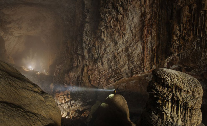
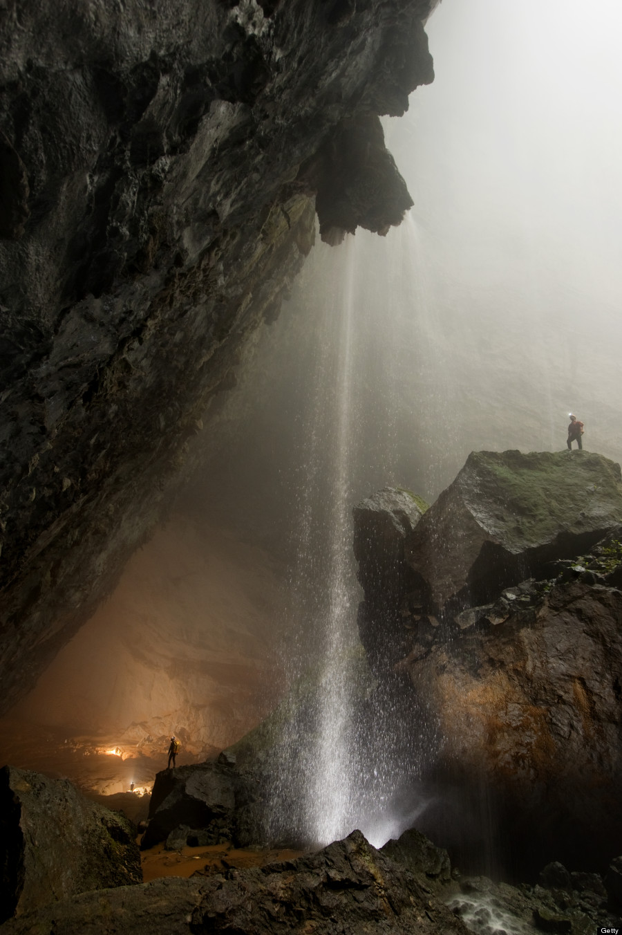
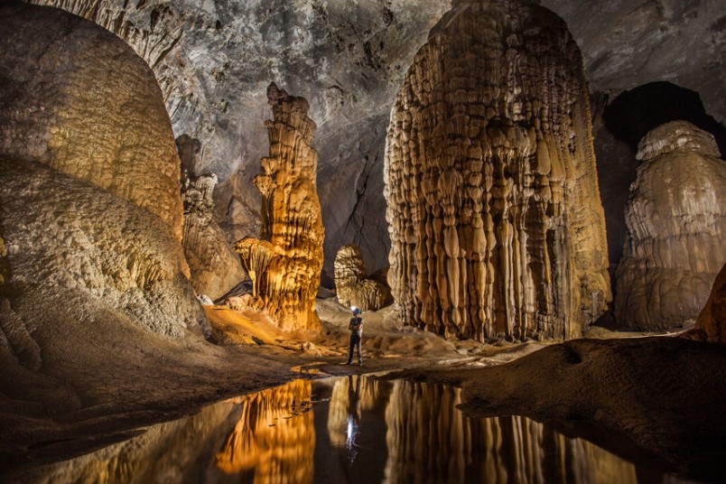
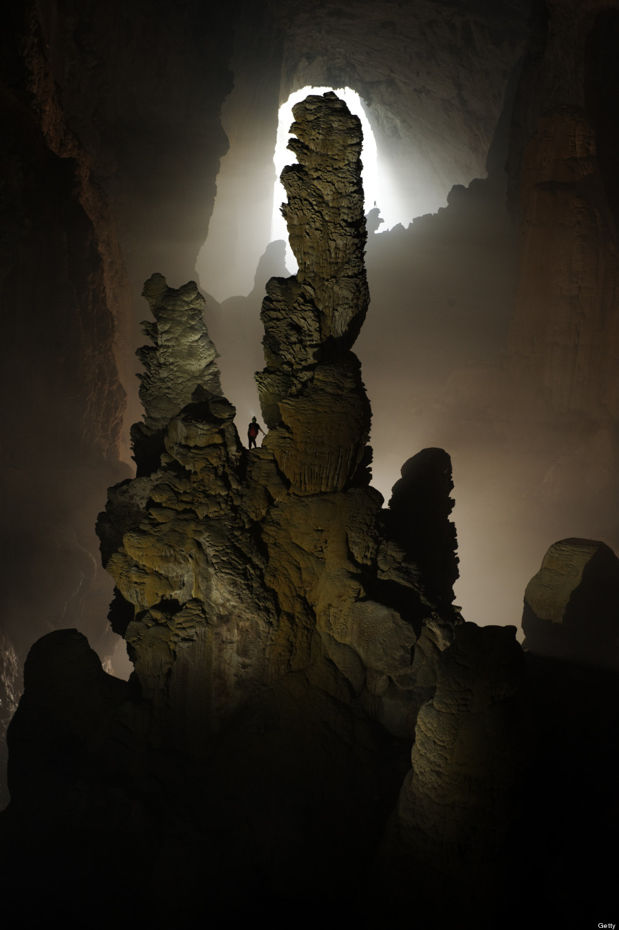
Krubera Cave is the deepest known cave on Earth. It is located in the Arabika Massif of the Gagra Range of the Western Caucasus, in the Gagra district of Abkhazia, a breakaway region of Georgia.
The difference in elevation of the cave’s entrance and its deepest explored point is 2,197 ± 20 metres (7,208 ± 66 ft). It became the deepest-known cave in the world in 2001 when the expedition of the Ukrainian Speleological Association reached a depth of 1,710 m (5,610 ft) which exceeded the depth of the previous deepest known cave, Lamprechtsofen, in the Austrian Alps, by 80 m. In 2004, for the first time in the history of speleology, the Ukrainian Speleological Association expedition reached a depth greater than 2,000 m, and explored the cave to −2,080 m (−6,824 ft). Ukrainian diver Gennadiy Samokhin extended the cave by diving in the terminal sump to 46 m depth in 2007 and then to 52 m in 2012, setting successive world records of 2,191 m and 2,197 m respectively. Krubera remains the only known cave on Earth deeper than 2,000 metres.
Location and background
Map of the Arabika Massif, showing the location of Krubera Cave and its projected resurgences
The Arabika Massif, the home of Krubera (Voronya) Cave, is one of the largest high-mountain limestone karst massifs in the Western Caucasus. It is composed of Lower Cretaceous and Upper Jurassic limestones that dip continuously southwest to the Black Sea and plunge below the modern sea level.
To the northwest, north, northeast, and east, Arabika is bordered by the deeply incised canyons of Sandripsh, Kutushara, Gega and Bzyb rivers. The Bzyb River separates Arabika from the adjacent Bzybsky Massif, another outstanding karst area with many deep caves, including the Snezhnaja-Mezhonogo-Iljuzia System (−1,753 m or −5,751 ft) and Pantjukhina Cave (−1,508 m or −4,948 ft). To the southwest, Arabika borders the Black Sea.
The Arabika Massif has a prominent high central sector with elevations above the tree line at ~1,800–1,900 m (5,900–6,200 ft). This is an area of classical glaciokarstic landscape, with numerous glacial trough valleys and cirques, with ridges and peaks between them. The bottoms of trough valleys and karst fields lie at elevations of 2,000–2,350 m (6,560–7,710 ft), and ridges and peaks rise to 2,500–2,700 m (8,200–8,900 ft). The highest peak is the Peak of Speleologists (2,705 m (8,875 ft)) but the dominant summit is a typical pyramidal horn of the Arabika Mount (2,695 m (8,842 ft)). Some middle- to low-altitude ridges covered with forest lie between the central sector and the Black Sea. A plateau-like middle-altitude outlier of the massif in its south sector is Mamzdyshkha, with part of the plateau slightly emerging above the tree line.
Among several hundred caves known in the Arabika Massif, fifteen have been explored deeper than 400 m and five deeper than 1,000 m (shown in Figure 1).
Krubera Cave is located at 2,256 m above sea level in the Ortobalagan Valley, a perfectly shaped, relatively shallow, glacial trough of the sub-Caucasian stretch, which holds the advanced position in the Arabika’s central sector relative to the seashore. Since 1980, Ukrainian cavers have been undertaking systematic efforts in exploring deep caves in the Ortobalagan Valley, resulting in exploration of the Krubera Cave to its current depth and of the Arabikskaja System to depth of −1,110 m (−3,640 ft). The latter consists of Kuybushevskaya Cave (also spelled as Kujbyshevskaja; −1,110 m) and Genrikhova Bezdna Cave (−965 m to the junction with Kujbyshevskaja). Another deep cave in the valley, located in its very upper part and explored by Moldavian and Ukrainian cavers is Berchilskaya Cave, 500 m (1,600 ft) deep. All large caves of the Ortobalagan Valley likely belong to a single hydrological system, connected to large springs at the Black Sea shore. The direct physical connection of Krubera Cave with the Arabikaskaja System is a sound possibility, although not yet physically realized.
Geology
Schema of caves Kruber-Voronija
The Ortobalagan Valley extends along the crest of the Berchil’sky anticline, which gently dips northwest. The cave entrances are aligned along the anticlinal crest but the caves are controlled by longitudinal, transverse, and oblique fractures and faults and comprise complex winding patterns in the plan view, remaining largely within and near the anticlinal crest zone. The caves are predominantly combinations of vadose shafts and steep meandering passages, although in places they cut apparently old fossil passages at different levels (e.g., at −2,100–2,040 m (−6,890–6,690 ft) in Kujbyshevskaja and Krubera caves, −1,200–1,240 m (−3,940–4,070 ft) and −980–1,150 m (−3,220–3,770 ft) in the non-Kujbyshevskaja branch of Krubera Cave, etc.). The deep parts of Krubera display a more pervasive conduit pattern with a mixture of phreatic morphology, characteristic of the zone of high-gradient floods, which can be up to 400 m above the low-flow water table, and vadose downcutting elements that are observed even below the water table.
The core part of the Arabika Massif is composed of the Upper Jurassic succession resting on the Bajocian Porphyritic Series, which includes sandstones, clays and conglomerates at the top, and tuff, tuff sandstones, conglomerates and breccia, porphyry and lava. The Porphyritic series forms the non-karstic basement of Arabika, which is exposed only on the northern and eastern outskirts, locally in the bottoms of the Kutushara and Gega River valleys. In the central part of Arabika the Cretaceous cover (Valanginian and Hauterivian limestones, marls and sandstones) is retained only in a few ridges and peaks, but it lies intact through the low-altitude ridges to the south-west of the central part. There the Cretaceous succession includes Barremian and Aptian–Cenomanian limestones and marly limestones with abundant concretions of black chert.
The Upper Jurassic succession begins with thin-bedded Kimmeridgian–Oxfordian cherty limestones, marls, sandstones and clays, which are identified in the lower part of Krubera Cave. Above lies the thick Tithonian succession of thick-bedded limestones with marly and sandy varieties. Sandy limestones are particularly abundant through the upper 1,000 m sections of deep caves of the Ortobalagan Valley.
The tectonic structure of Arabika is dominated by the axis of the large sub-Caucasian anticline (oriented NW–SE), with the gently dipping southwestern mega-flank, complicated by several low-order folds, and steeply dipping northeastern flank (Figure 3). The axis of the anticline roughly coincides with the ridge bordering the Gelgeluk Valley to the north. Located on the southwestern flank of the major anticline is another large one (Berchil’sky), in which the crest is breached by the Ortobalagan Valley. There are several smaller sub-parallel anticlines and synclines farther southwest, between the Berchil’ Ridge and the coast.
The plicative dislocation structure of the massif is severely complicated by faults, with the fault-block structure strongly controlling both cave development and groundwater flow. Major faults of the sub-Caucasian orientation delineate several large elongated blocks that experienced uplift with different rates during Pliocene and Pleistocene. This had a pronounced effect on the development of deep groundwater circulation and of Krubera Cave in particular. Both longitudinal and transverse faults and related fracture zones play a role in guiding groundwater flow; the latter guide flow across the strike of major plicative dislocations, from the central sector toward the Black Sea.
Hydrogeology
Major on-shore karst springs with individual average discharges of 1 to 2.5 m3/s (35 to 88 cu ft/s) are located at altitudes ranging from 1 m (3.3 ft) (Reproa Spring) to 540 m (1,770 ft) (Gega waterfall). Two of them are located in the shore area; these are Reproa (average discharge 2.5 m3/s or 88 cu ft/s; altitude 1 m or 3 ft 3 in above sea level) and Kholodnaja Rechka (1.2 m3/s or 42 cu ft/s; 50 m or 160 ft a.s.l.). Two more major springs are located in the river canyons bordering Arabika to the east: Goluboe Ozero in the Bzyb canyon (2.5 m3/s or 88 cu ft/s; 90 m or 300 ft a.s.l.) and Gega waterfall in the Gega canyon (1 m3/s or 35 cu ft/s; 540 m or 1,770 ft a.s.l.). There are also several smaller springs in the Gagra town.
Some boreholes located along the shore of the Black Sea yield karstic groundwater from depths of 40–280 m below sea level. Other much deeper boreholes tapped low-salinity karstic waters at depths of 500 and 1,750 m in the Khashupse Valley near Tsandripsh and 2,250 m near Gagra. This suggests the existence of a deep karst system and vigorous karst groundwater circulation at depth.
Submarine springs are known in the Arabika area, emerging from the floor of the Black Sea in front of the massif. Shallow springs at depths of 5–7 m can be reached by free dive near Tsandripsh. Tamaz Kiknadze (1979) reported submarine springs near the eastern part of Gagra at depth of 25–30 m and Buachidze and Meliva (1967) revealed submarine discharge at depths up to −400 m by hydrochemical profiling. Recently an outstanding feature of the sea floor topography near Arabika has been revealed from a digital bathymetric map that combines depth soundings and high-resolution marine gravity data. This is a huge submarine depression in front of the Zhovekvara River mouth, which has dimensions of about 5 x 9 km and a maximum depth of about 380 m (1,250 ft). The Arabika Submarine Depression is a closed feature with internal vertical relief of about 120 m (390 ft) (measured from its lowest rim) separated from the abyssal slope by the bar at a depth of about 260 m (850 ft). It has steep northern and northeastern slopes (on the side of the massif) and gentle south and southwestern slopes. Its formation is apparently karstic. Presently this depression seems to be a focus of submarine discharge of the karst systems of Arabika.
The speleological explorations and a series of dye tracing experiments conducted during the 1980s under the coordination of Alexander Klimchouk have radically changed previous notions of the hydrogeology of Arabika, revealed its outstanding speleological perspectives and strongly stimulated further efforts for exploration of deep caves. Tracers injected in the Kujbyshevskaja Cave and the Iljukhina System were detected in the Kholodnaja Rechka and Reproa springs, proving groundwater flow to the south-southwest across major tectonic structures over a distance of 13–16 km as the crow flies (Figure 1). The tracer from Kujbyshevskaja Cave was also detected in a borehole located between these two springs, which yields groundwater from a depth of 200 m (660 ft) below sea level. This has been interpreted as an indication of the connection of the cave with the submarine discharge. The large “Central Karst Hydrologic System”, which encompasses most of the southeastern flank of the Arabika anticline, had been identified in this way. The system became the deepest in the world with its overall vertical range of about 2,500 m (8,200 ft) (measuring to the borehole water-bearing horizon) or even 2,700 m (8,900 ft) (measuring to the deepest reported submarine discharge points).
Another tracer was injected in the Moskovskaja Cave (−970 m) and detected at the Gegsky Vodopad spring, indicating the presence of a karst hydrologic system comprising the northeastern flank of the Arabika anticline (the “Northern System”). No connections have been revealed with yet another major spring, Goluboje Ozero in the Bzyb River canyon, although it apparently drains a large area of the eastern sector of the massif (the hypothetical “Eastern Karst Hydrological System”). It is not clear where Sarma Cave (−1,550 m) drains to, Goluboje Ozero to the southeast or Reproa to the southwest, at the shore.
The results of the dye-tracing tests demonstrated that groundwater flow is not subordinate to the fold structure but is largely controlled by faults that cut across the strike of major folds, and that the large part of the central sector of Arabika is hydraulically connected to the springs along the seashore and with submarine discharge points.
Krubera Cave has an extremely steep profile and reveals a huge thickness of the vadose zone. The lower boundary of the vadose zone (the top of the phreatic zone) is at an elevation of about 110 m (360 ft) at low flow, which suggests a low overall hydraulic gradient of 0.007-0.008. Low-TDS groundwater is tapped by boreholes in the shore area at depths of 40–280, 500, 1,750, and 2,250 m below sea level, which suggests the existence of a deep flow system with vigorous flow. Submarine discharge along the Arabika coast is reported at depths up to ~400 m b.s.l.
It is difficult to interpret these facts in terms of the development of karst systems controlled by contemporary sea level, or within the range of its Pleistocene fluctuations (up to −150 m). In combination with the existence of the Arabika Submarine Depression, all these facts point to the possibility that karst systems in Arabika could have originated in response to the Messinian salinity crisis (5.96–5.33 Ma) when the Black Sea (Eastern Paratethys) could have almost dried up, as did the adjacent Mediterranean, where the dramatic sea level drop of ~1,500 m is well established.
Scanning electron microscope image of a shock-metamorphosed zircon from the Sudbury impact crater, Ontario, Canada. The parallel planar fractures are caused by the extreme conditions of the impact itself while the anastomosing cracks represent later damage. The zircon is less than 0.1 mm wide. Credit: Gavin Kenny, Trinity College Dublin, in Geology.
In this new article for Geology, Gavin Kenny and colleagues reveal the likely origin of Earth’s oldest crystals. New research into the origin of Earth’s oldest crystals suggests that they probably formed in huge impact craters rather than during the collision of tectonic plates moving around on Earth’s surface as had previously been thought.
With very few rocks preserved from Earth’s early history, the only material geoscientists have from this time comes in the form of tiny, naturally occurring crystals known as zircons. Naturally then, the origin of these crystals, which are approximately the width of a human hair, are more than four billion years old, and have famously suggested the presence of water on the very early Earth, has become a matter of major debate.
In this latest breakthrough, scientists from Trinity College, Dublin, and the Swedish Museum of Natural History, Stockholm, have shown that zircon crystals that formed in a much younger impact crater are indistinguishable from the very ancient zircons from early Earth. Given the fact that our planet suffered more asteroid impacts early on than it has in relatively recent times, this strongly suggests that many of the oldest crystals known to man could have formed in violent impact crater settings.
Reference:
Gavin G. Kenny et al., Differentiated impact melt sheets may be a potential source of Hadean detrital zircon. DOI: 10.1130/G37898.1
This is a left lower jaw of Yunnanadapis folivorus, one of six new fossil species found in southern China. Credit: Courtesy IVPP, Chinese Academy of Sciences; also courtesy University of Kansas
In a study to be published this week in the journal Science, researchers describe unearthing a “mother lode” of a half-dozen fossil primate species in southern China.
These primates eked out an existence just after the Eocene-Oligocene transition, some 34 million years ago. It was a time when drastic cooling made much of Asia inhospitable to primates, slashing their populations and rendering discoveries of such fossils especially rare.
“At the Eocene-Oligocene boundary, because of the rearrangement of Earth’s major tectonic plates, you had a rapid drop in temperature and humidity,” said K. Christopher Beard, senior curator at the University of Kansas’ Biodiversity Institute and co-author of the report. “Primates like it warm and wet, so they faced hard times around the world — to the extent that they went extinct in North America and Europe. Of course, primates somehow survived in Africa and Southern Asia, because we’re still around to talk about it.” Because anthropoid primates — the forerunners of living monkeys, apes and humans– first appeared in Asia, understanding their fate on that continent is key to grasping the arc of early primate and human evolution.
“This has always been an enigma,” Beard said. “We had a lot of evidence previously that the earliest anthropoids originated in Asia. At some point, later in the Eocene, these Asian anthropoids got to Africa and started to diversify there. At some point, the geographic focal point of anthropoid evolution — monkeys, apes and humans — shifted from Asia to Africa. But we never understood when and why. Now, we know. The Eocene-Oligocene climate crisis virtually wiped out Asian anthropoids, so the only place they could evolve to become later monkeys, apes and humans was Africa.”
The paper is the product of a decade’s worth of fieldwork at a site in southern China, where the primates likely sought warmer temperatures. Beard and his colleagues Xijun Ni, Qiang Li and Lüzhou Li of the Chinese Academy of Sciences’ Institute of Vertebrate Paleontology and Paleoanthropology describe the six new species from jaw and tooth fragments, which survived the ages due to their tough enamel surfaces and serve as “fingerprints” to identify ancient animals.
“The fossil record usually gives you a snapshot here or there of what ancient life was like. You typically don’t get a movie,” Beard said. “We have so many primates from the Oligocene at this particular site because it was located far enough to the south that it remained warm enough during that cold, dry time that primates could still survive there. They crowded into the limited space that remained available to them.”
Like most of today’s primates, the KU researcher said the ancient Chinese primates were tropical tree-dwellers. One of the species, which the research team has named Oligotarsius rarus, was “incredibly similar” to the modern tarsier found today only in the Philippine and Indonesian islands.
“If you look back at the fossil record, we know that tarsiers once lived on mainland Asia, as far north as central China,” Beard said. “The fossil teeth described in this paper are nearly identical to those of modern tarsiers. Research shows that modern tarsiers are pretty much living fossils — those things have been doing what they do ever since time immemorial, as far as we can tell.”
Beard said that if not for the intense global cooling of the Eocene-Oligocene transition, the main stage of primate evolution may have continued to be in Asia, rather than transitioning to Africa where Homo sapiens eventually emerged. Indeed, the team’s findings underscore a vulnerability to climate change shared by all primates.
“This is the flip side of what people are worried about now,” he said. “The Eocene-Oligocene transition was the opposite of global warming — the whole world was already warm, then it cooled off. It’s kind of a mirror image. The point is that primates then, just like primates today, are more sensitive to a changing climate than other mammals.”
Reference:
Xijun Ni, Qiang Li, Lüzhou Li, K. Christopher Beard. Oligocene primates from China reveal divergence between African and Asian primate evolution. Science, 2016 DOI: 10.1126/science.aaf2107
A graphic illustrating seismic zones and activity in New Zealand. The figure on the bottom right shows the horizontal and vertical movement caused by a slow-slip event. Credit: GNS Science/Laura Martin
Research published in the May 6 edition of Science indicates that slow-motion earthquakes or “slow-slip events” can rupture the shallow portion of a fault that also moves in large, tsunami-generating earthquakes. The finding has important implications for assessing tsunami hazards. The discovery was made by conducting the first-ever detailed investigation of centimeter-level seafloor movement at an offshore subduction zone.
“These data have revealed the true extent of slow-motion earthquakes at an offshore subduction zone for the first time,” said Laura Wallace, a research scientist at The University of Texas at Austin’s Institute for Geophysics who led the study.
An international team of researchers from the U.S., Japan and New Zealand collaborated on the research. The Institute for Geophysics is a research unit of The University of Texas Jackson School of Geosciences.
The world’s most devastating tsunamis are generated by earthquakes that occur near the trenches of subduction zones, places where one tectonic plate begins to dive or “subduct” beneath another. Using a network of highly sensitive seafloor pressure recorders, the team detected a slow-slip event in September 2014 off the east coast of New Zealand. The study was undertaken at the Hikurangi subduction zone, where the Pacific Plate subducts beneath New Zealand’s North Island.
The slow-slip event lasted two weeks, resulting in 15-20 centimeters of movement along the fault that lies between New Zealand and the Pacific Plate, a distance equivalent to three to four years of background plate motion. If the movement had occurred suddenly, rather than slowly, it would have resulted in a magnitude 6.8 earthquake. The seafloor sensors recorded up to 5.5 centimeters of upward movement of the seafloor during the event.
Slow-slip events are similar to earthquakes, but instead of releasing strain between two tectonic plates in seconds, they do it over days to weeks, creating quiet, centimeter-sized shifts in the landscape. In a few cases, these small shifts have been associated with setting off destructive earthquakes, such as the magnitude 9.0 Tohoku-Oki earthquake that occurred off the coast of Japan in 2011 and generated a tsunami that caused the Fukushima Daiichi nuclear power plant disaster.
The slow-slip event that the team studied occurred in the same location as a magnitude 7.2 earthquake in 1947 that generated a large tsunami. The finding increases the understanding of the relationship between slow slip and normal earthquakes by showing that the two types of seismic events can occur on the same part of a plate boundary.


The link has been difficult to document in the past because most slow-slip monitoring networks are land-based and are located far from the trenches that host tsunami-generating earthquakes, Wallace said. The data for this study was recorded by HOBITSS, a temporary underwater network that monitored slow-slip events by recording vertical movement of the seafloor. HOBITSS stands for “Hikurangi Ocean Bottom Investigation of Tremor and Slow Slip.”
“Our results clearly show that shallow, slow-slip event source areas are also capable of hosting seismic rupture and generating tsunamis,” said Yoshihiro Ito, a professor at Kyoto University and study co-author. “This increases the need to continuously monitor shallow, offshore slow-slip events at subduction zones, using permanent monitoring networks similar to those that have been established offshore of Japan.”
Professor Spahr Webb, a co-author from Columbia University’s Lamont-Doherty Earth Observatory agreed.
“Our New Zealand experiment results demonstrate the great potential for using offshore monitoring systems at subduction zones in the Pacific Northwest for tsunami and earthquake early warning,” said Webb.
Earthquakes are unpredictable events, Wallace said, but the linkage between slow-slip events and earthquakes could eventually help in forecasting the likelihood of damaging earthquakes.
“To do that we will have to understand the links between slow-slip events and earthquakes much better than we currently do,” Wallace said.
The research team installed the HOBITSS network in May 2014, which consisted of 24 seafloor pressure gauges, and 15 ocean bottom seismometers. The team collected the devices and data in June 2015.
“The project findings add to critical information for anticipating potentially life-threatening earthquakes and tsunamis,” said Maurice Tivey, program director of the National Science Foundation’s Division of Ocean Sciences.
Reference:
“Slow slip near the trench at the Hikurangi subduction zone, New Zealand,” Science, DOI: 10.1126/science.aaf2349
Puerto Rico’s Mameyes River experiences frequent flash floods in which water discharge can increase 100-fold over normal levels. These images of the same section of river (with the identical tree marked in each for reference) show how dramatically river flow can change. Yet a study by researchers from the University of Pennsylvania shows that these events have a much smaller contribution to erosion than might be expected. Credit: Colin Phillips
In the Puerto Rican rain forest, a strong storm can drop a meter of rain in a single day. All that water rushes into mountain rivers and causes a torrent as the water overflows the riverbanks and charges downstream.
It seems intuitive that the force of so much water would lead to massive erosion of a riverbed. But according to a new study by University of Pennsylvania researchers, that intuition is incorrect.
The work, published in the journal Science, shows that, though extreme precipitation events can greatly increase the amount of water traveling through a river, large storms only move about 50 percent more sediment than a typical rainfall. The overall contribution of these intense rainfalls to erosion, therefore, is smaller than might be expected.
With climate change expected to bring more intense precipitation in many regions of the globe, the findings indicate that, while these extreme rainfall events may at first lead to more flooding, river channels may rapidly increase their size to accommodate the flow.
“Our work suggests that river channels may set the speed limit on erosion,” said Douglas J. Jerolmack, associate professor in Penn’s Department of Earth and Environmental Science in the School of Arts & Sciences. “We showed that the forces of the biggest flood events were really only incrementally larger than the moderate events because river channels adjust their size to be close to the so-called ‘threshold of motion,’ or the force required to move particles on the riverbed.”
The research was conducted by Jerolmack and his former graduate student Colin Phillips. Phillips is now a postdoctoral researcher at the University of Minnesota.
The work began with an investigation of the Mameyes River in the Luquillo Critical Zone Observatory in northeastern Puerto Rico, where flash floods are common. The researchers set out to determine how often and how far particles on the riverbed moved in response to rainfall. They placed RFID tags inside 350 grapefruit-sized cobbles on the riverbed and then checked on their location after numerous rains during the course of two years. They also monitored the force of the river water using a United States Geological Survey stream gage near their study site.
They found that rainfall events strong enough to move the cobbles occurred about 20 times a year. But, though the heaviest rainfalls could increase the river discharge 100-fold, these storms moved the tracers only moderately farther than a more typical rain.
Surprised by their findings on the Mameyes, Phillips and Jerolmack set out to determine whether the same would be true of rivers generally. To do so, they gathered USGS data from 186 rivers for which they had information on the width, depth and sediment type of the river and records of the river discharge through time.
Analyzing these data, they confirmed that, for rivers transporting gravel-sized and larger coarse material, flows exceeding the threshold of motion were rare.
While some rivers experience flows at the threshold of motion many times per year and others only once every few years, the scientists found a repeating pattern for flows above threshold.
“Not only did we find that they were very rare but that the distribution of forces that exceed the critical force to move particles was the same for all of the rivers that we looked at,” Jerolmack said.
In other words, they found that flows that were 1.5 times threshold were 100 times less frequent than threshold floods, and flows 2 times threshold were 100 times less frequent than that.
The reason for this commonality, according to the researchers, is that the width and depth of river channels adjust to keep the forces of water flow near the threshold of motion.
“The argument is that, if the sediment transport rate during a flood was too high,” Jerolmack said, “the river bank would erode and the channel would widen. If the channel widened, then the depth of the flow would drop and that would bring the force on the river bed back down. There is this regulation mechanism that ensures the river channel is just the size it needs to be.”
As many landscape models have operated under the assumption that more variable rainfall equates with more erosion, the findings will likely trigger a new look at the connection between climate change and landscape change.
“Any time you can find something general and common in the messy world out there, it’s a useful finding,” Jerolmack said. “It allows us to simplify our models for predicting river erosion and its response to climate.”
While these results apply to rivers with gravel and larger-sized particles, the researchers hope to extend their work to determine the properties that govern erosion by rivers that have sand and mud, which may be different.
Reference:
“Self-organization of river channels as a critical filter on climate signals,” Science, DOI: 10.1126/science.aad3348
The fossil chelicerate larva discovered by LMU researchers is only 2 mm
On the basis of an analysis of 520 million-year-old fossils, LMU researchers show that embryonic and larval development in the early ancestors of spiders and scorpions was strikingly and unexpectedly similar to that of modern crabs.
The shale formations of Chengjiang in southwestern China are a treasure trove for palaeontologists and evolutionary biologists. The fossils found there are over half a billion years old, and researchers have been excavating them since the 1980s. The specimens that have come to light are so diverse and, for the most part, so well preserved that they provide scientists with a very detailed picture of what animals looked like in the Early Cambrian. This was the period in Earth’s history when most of the major groups of animals represented in the biosphere today first evolved. Together with colleagues from Germany, China and the US, and with the aid of novel methods, LMU researchers have now obtained new insights into the evolution of ontogeny – the developmental process that leads to the transition from embryo to adult – in the taxon Arthropoda, an extremely diverse and abundant group of animals today, which includes the insects, spiders, centipedes and crustaceans. The new findings appear in the “Proceedings of the U.S. National Academy of Sciences”.
Dr. Yu Liu (Department of Biology II, currently Department of Earth & Environmental Science at LMU) and his colleagues are well acquainted with fossil specimens of the species Leanchoilia illecebrosa. This arthropod is thought to represent an early marine form of the chelicerates, the group that includes spiders, scorpions and mites, as well as the horseshoe “crab” Limulus polyphemus (which – unlike the true crabs – is not a crustacean). The adult representatives of L. illecebrosa previously analyzed by the Munich researchers were between 2 and 4 cm long, and they described an immature larva two years ago that measures only about 8 mm in length. In this new paper they report a fossil that is only 2 mm long and carries a pair of pincer-like appendages, each comprising three flagella-like elements together with four pairs of well-developed branched limbs in the head, and a spike-like posterior region or telson. The authors interpret this specimen as an even earlier larval stage of Leanchoilia.
New segments at a specialized growth zone
Some aspects of the new fossil surprised Yu Liu and his colleagues, because they do not conform to the pattern of development that would be expected for an early representative of the chelicerates, based on what is known about the evolutionary pathway that led to modern arthropods. For instance, the new larva has fewer body segments than the adult, and the limbs at the rear of the trunk are rudimentary. To the LMU team (which also included Prof. Dr. Roland Melzer, Dr. Joachim Haug and Dr. Carolin Haug of the Department Biology II) and their colleagues, these features are more reminiscent of the later larval stages of modern crustaceans. In crustaceans, only the first four segments are fully developed in the newly hatched larva. New segments are progressively added to the trunk at a specialized growth zone located just in front of the telson over the course of several further larval stages. For the scientists, the new specimen of L. illecebrosa is yet another example of how important it is “to consider not only the morphology of mature organisms, but also their development from embryo to adult,” i.e. the ontogenetic patterns, when reconstructing the evolution of animal groups.
The kind of detailed analysis carried out on this mini-larva “was made possible by a combination of several high-end methodologies,” says Yu Liu. Among other techniques, the team subjected samples of the shale to computerized microtomography (micro-CT). This permits investigators to reconstruct and examine the fossil in three dimensions, without the need to painstakingly remove the sedimentary material concealing it.
Reference:
Yu Liu et al. Three-dimensionally preserved minute larva of a great-appendage arthropod from the early Cambrian Chengjiang biota, Proceedings of the National Academy of Sciences (2016). DOI: 10.1073/pnas.1522899113
Fig.2 A Sketch reconstruction of the fish-eating enantiornithine bird. Credit: WANG Min and SHI Aijuan
Enantiornithes are the most successful clade of Mesozoic birds, representing the sister group of the Ornithuromorpha, which gave rise to living birds. Nevertheless, the feeding habits of enantiornithines have remained unknown because of a lack of fossil evidence. In contrast, exceptionally preserved fossils reveal that derived avian features were present in the digestive systems of some non-enantiornithine birds with ages exceeding 125 million years.
In paper published online April 28 in the journal of Current Biology (26), Drs. WANG Min, ZHOU Zhonghe and Corwin Sullivan, Institute of Vertebrate Paleontology and Paleoanthropology (IVPP ), Chinese Academy of Sciences, reported a new piscivorous enantiornithine from the Early Cretaceous Jehol Biota of China. This specimen preserves a gastric pellet that includes fish bones, and is the oldest birds’ pellet dating back 120 million years ago. This finding provides evidence of modern avian digestive features in the Early Cretaceous enantiornithine birds.
The new enantiornithine bird (IVPP V22582) was collected from the Lower Cretaceous Jiufotang Formation near Dapingfang Town, Chaoyang Country, Liaoning Province, northeastern China. It was assigned to Enantiornithes on a combination of characteristics including the coracoid lacking a procoracoid process and having a convex lateral margin. A detailed morphological study of the new specimen is in preparation and will be presented in a separated paper.
Modern birds differ from their theropod ancestors in lacking teeth and heavily constructed bony jaws, having evolved a lightly built beak and a specialized digestive system capable of processing unmasticated food.
Researchers observed that a spindle-shaped cluster of fish bones, with long and short axes measuring 22.6 mm and 7.1 mm respectively, is overlapped by the right humerus. The bones include vertebrae, neural spines, and unidentifiable fragments. They are most likely attributable to the teleost Lycoptera, the most abundant fish at this locality.
Researchers believed that the spindle-shaped structure was a pellet regurgitated by the bird shortly before, or even at, the time of death. This conclusion is reinforced by the sharp boundary between the brown matrix enclosing the densely concentrated fish bones and the white host matrix of the slab, which implies that the spindle-shaped structure was cohesive and well defined like the pellets of modern birds. Because of these characteristics and the lack of fish bones elsewhere on the slab, the aggregation is unlikely to be a preservational artifact.
This new enantiornithine, like many modern piscivores and raptors, seems to have swallowed its prey whole and regurgitated indigestible materials such as bones, invertebrate exoskeletons, scales, and feathers. This finding provides the first evidence that some enantiornithine birds were piscivorous and that distinctive features of modern avian digestive system were well established in some Early Cretaceous birds.
“This fossil represents the oldest unambiguous record of an avian gastric pellet and the only such record from the Mesozoic”, said lead author WANG Min of the IVPP, “The pellet points to a fish diet and suggests that the alimentary tract of the new enantiornithine resembled that of extant avians in having efficient antiperistalsis and a two-chambered stomach with a muscular gizzard capable of compacting indigestible matter into a cohesive pellet.”
“The inferred occurrence of these advanced features in an enantiornithine implies that they were widespread in Cretaceous birds and likely facilitated dietary diversification within both Enantiornithes and Ornithuromorpha”, said ZHOU Zhonghe, co-correspoding author of the IVPP.
Painted Hills, in the northwest United States, is one of the three units of the John Day Fossil Beds National Monument, located in Wheeler County, Oregon.
It totals 3,132 acres (12.67 km2) and is located 9 miles (14 km) northwest of Mitchell, Oregon. The Painted Hills are listed as one of the Seven Wonders of Oregon.
Painted Hills is named after the colorful layers of its hills corresponding to various geological eras, formed when the area was an ancient river floodplain.
The black soil is lignite that was vegetative matter that grew along the floodplain. The grey coloring is mudstone, siltstone, and shale. The red coloring is laterite soil that formed by floodplain deposits when the area was warm and humid.
An abundance of fossil remains of early horses, camels, and rhinoceroses in the Painted Hills unit makes the area particularly important to vertebrate paleontologists.
Rio Tinto’s Argyle Pink Diamonds business has unveiled the largest violet diamond recovered from the Argyle mine in Western Australia.
The 2.83 carat polished oval shaped diamond, known as The Argyle Violet, will be the dazzling centrepiece of the 2016 Argyle Pink Diamonds Tender, the annual showcase of the rarest diamonds from the Argyle mine.
Argyle Pink Diamonds manager Josephine Johnson said “We are very excited to announce this historic diamond ahead of our Tender launch. This stunning violet diamond will capture the imagination of the world’s leading collectors and connoisseurs.”
More than 90 per cent of the world’s rare pink diamonds com from the Argyle mine and it is the only source of hydrogen-rich violet diamonds. Violet diamonds are seldom seen and in 32 years Argyle has produced only 12 carats of polished violet diamonds for its iconic Tender.
The Argyle Violet was polished in Western Australia by one of Argyle’s master polishers, Richard How Kim Kam, from a 9.17 carat rough diamond discovered in 2015. The Argyle Violet has been assessed by the Gemological Institute of America (GIA) as a notable diamond with the colour grade of Fancy Deep Greyish Bluish Violet.
Rio Tinto Diamonds general manager of sales, Patrick Coppens said “Impossibly rare and limited by nature, The Argyle Violet will be highly sought after for its beauty, size and provenance.”
The 2016 Argyle Pink Diamonds Tender will commence private trade viewings in June and travel to Copenhagen, Hong Kong and New York.
This molecular phylogeny of scarab beetles was dated to provide the first molecular evidence that dung beetles evolved in association with dinosaurs. Credit: Laura Dempsey/Cleveland Museum of Natural History
Researchers have found an evolutionary connection between dinosaurs and dung beetles. An international team of scientists uncovered the first molecular evidence indicating that dung beetles evolved in association with dinosaurs. The findings place the origin of dung beetles (Scarabaeidae: Scarabaeinae) in the Lower Cretaceous period, with the first major diversification occurring in the middle of the Cretaceous. This timeline places their origins approximately 30 million years earlier than previously thought. The research explores the potential of a co-extinction with dinosaurs 66 million years ago. The study was published today in the open-access journal PLOS ONE.
Lead author Dr. Nicole Gunter of The Cleveland Museum of Natural History generated molecular (DNA) sequence data from 125 scarab beetles at the Australian National Insect Collection, CSIRO, which were aligned with previously published data to create a total dataset representing 450 beetle species. The data were used to create a dated molecular phylogeny of scarab beetles. Analyses compared timing and evolutionary relationships of herbivorous scarab subfamilies that feed directly on living plant tissue to saprophagous scarab subfamilies that feed on dead and decaying matter–including dung.
The results confirmed that the evolution of herbivorous scarab beetles tracked the ecological dominance of flowering plants, or angiosperms. Interestingly, the dung beetles also underwent a similar diversification pattern as the herbivorous scarabs, providing the first evidence of indirect influence of angiosperms on non-herbivorous insects. The study places the evolution of dung beetles at about 115 to 130 million years ago in the Lower Cretaceous.
“Surprisingly, the timing and diversification of dung beetles is correlated with the ecological dominance of angiosperms,” said lead author Dr. Nicole Gunter, invertebrate zoology collections manager at The Cleveland Museum of Natural History. “Through these findings, we hypothesize that the incorporation of flowering plants in the diet of dinosaurs resulted in the first palatable dung source for feeding–providing a new niche for evolution.”
“Dinosaurs were the dominant terrestrial animals for 135 million years and definitely shaped ecosystems throughout their existence,” said co-author Dr. Stephen Cameron of Queensland University of Technology in Australia. “This paper is the first to demonstrate that the speciation of a group was tied to utilizing dinosaurs as an ecological resource–their dung.” The scientists note the existence of dinosaur coprolites (fossilized feces) showing evidence of tunneling attributed to dung beetle feeding dated at 70 to 80 million years ago, which is in line with the new hypothesis on dung beetle evolution outlined in this new study.
“This research provides evidence supporting an extinction of dung beetles approximately 60 to 70 million years ago that can be readily associated with the Cretaceous-Paleogene mass extinction of non-avian dinosaurs,” said Gunter. “Our findings suggest that the loss of dinosaurs and their dung impacted dung beetle diversification–fortunately, they survived the extinction event. We hypothesize that modern dung beetles are descended from species that fed either on the dung of dinosaurs and early mammals, or species already adapted to feeding on Cretaceous mammal dung. We hope that this research brings attention to invisible extinctions not captured in the fossil record.”
Although the findings challenge previous research that associates the origin of dung feeding with mammals, this study also indicates dung beetles diversified at their greatest rate in the Paleogene in line with the major diversification of mammals. The team suggests that additional research is needed to disentangle the causes of the most recent diversification and to shed more light on the survival of dung beetles through the Cretaceous-Paleogene mass extinction. This story of dinosaurs, flowering plants, mammals and scarab beetles demonstrates the complex interactions of evolving ecosystems and that it is possible to determine the drivers of diversification, even for insects where the limited fossil record provides little insight into Cretaceous life.
Video
Reference:
Nicole L. Gunter, Tom A. Weir, Adam Slipinksi, Ladislav Bocak, Stephen L. Cameron. If Dung Beetles (Scarabaeidae: Scarabaeinae) Arose in Association with Dinosaurs, Did They Also Suffer a Mass Co-Extinction at the K-Pg Boundary? PLOS ONE, 2016; 11 (5): e0153570 DOI: 10.1371/journal.pone.0153570