Deadly snakes are among Australia’s most iconic animals. Now a new study led by The Australian National University (ANU) has helped explain how they descended from creatures that have come from Asia over the past 30 million years.
Lead researcher Dr Paul Oliver said about 85 per cent of more than 1,000 snake and lizard species in Australia descended from creatures that floated across waters from Asia to Australia.
The research helps explain how Australia has become home to about 11 per cent of the world’s 6,300 reptile species — the highest proportion of any country around the world.
“Around 30 million years ago it appears that the world changed, and subsequently there was an influx of lizard and snakes into Australia,” said Dr Oliver from the ANU Research School of Biology.
“We think this is linked to how Australia’s rapid movement north, by continental movement standards, has changed ocean currents and global climates.”
The researchers conducted the study using animal tree-of-life data combined with empirical evidence and simulations.
The origins for reptiles contrast with other famous Australian animal groups including marsupials and birds, which include many more species descended from ancestors that lived on Gondwana, a super continent that included Australia, Antarctica, South America, Africa and Madagascar.
Dr Oliver said that the study found that the immigration of reptiles into Australia was clustered in time.
“The influx of lizards and snakes into Australia corresponds with a time when fossil evidence suggests animal and plant communities underwent major changes across the world,” he said.
“The movement of Australia may have been a key driver of these global changes.”
The research is published in the Nature Ecology and Evolution.
Reference:
Paul M. Oliver, Andrew F. Hugall. Phylogenetic evidence for mid-Cenozoic turnover of a diverse continental biota. Nature Ecology & Evolution, 2017; DOI: 10.1038/s41559-017-0355-8
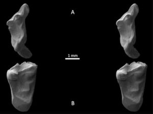
These are fossil teeth under electron microscope. Credit: University of Portsmouth
Fossils of the oldest mammals related to humankind have been discovered on the Jurassic Coast of Dorset.
The two teeth are from small, rat-like creatures that lived 145 million years ago in the shadow of the dinosaurs. They are the earliest undisputed fossils of mammals belonging to the line that led to human beings.
They are also the ancestors to most mammals alive today, including creatures as diverse as the Blue Whale and the Pigmy Shrew. The findings are published in the Journal, Acta Palaeontologica Polonica, in a paper by Dr Steve Sweetman, Research Fellow at the University of Portsmouth, and co-authors from the same university. Dr Sweetman, whose primary research interest concerns all the small vertebrates that lived with the dinosaurs, identified the teeth but it was University of Portsmouth undergraduate student, Grant Smith who made the discovery.
Dr Sweetman said: “Grant was sifting through small samples of earliest Cretaceous rocks collected on the coast of Dorset as part of his undergraduate dissertation project in the hope of finding some interesting remains. Quite unexpectedly he found not one but two quite remarkable teeth of a type never before seen from rocks of this age. I was asked to look at them and give an opinion and even at first glance my jaw dropped!”
“The teeth are of a type so highly evolved that I realised straight away I was looking at remains of Early Cretaceous mammals that more closely resembled those that lived during the latest Cretaceous — some 60 million years later in geological history. In the world of palaeontology there has been a lot of debate around a specimen found in China, which is approximately 160 million years old. This was originally said to be of the same type as ours but recent studies have ruled this out. That being the case, our 145 million year old teeth are undoubtedly the earliest yet known from the line of mammals that lead to our own species.”
Dr Sweetman believes the mammals were small, furry creatures and most likely nocturnal. One, a possible burrower, probably ate insects and the larger may have eaten plants as well.
He said: “The teeth are of a highly advanced type that can pierce, cut and crush food. They are also very worn which suggests the animals to which they belonged lived to a good age for their species. No mean feat when you’re sharing your habitat with predatory dinosaurs!”
The teeth were recovered from rocks exposed in cliffs near Swanage which has given up thousands of iconic fossils. Grant, now reading for his Master’s degree at The University of Portsmouth, said that he knew he was looking at something mammalian but didn’t realise he had discovered something quite so special. His supervisor, Dave Martill, Professor of Palaeobiology, confirmed that they were mammalian, but suggested Dr Sweetman, a mammal expert should see them.
Professor Martill said: “We looked at them with a microscope but despite over 30 years’ experience these teeth looked very different and we decided we needed to bring in a third pair of eyes and more expertise in the field in the form of our colleague, Dr Sweetman.
“Steve made the connection immediately, but what I’m most pleased about is that a student who is a complete beginner was able to make a remarkable scientific discovery in palaeontology and see his discovery and his name published in a scientific paper. The Jurassic Coast is always unveiling fresh secrets and I’d like to think that similar discoveries will continue to be made right on our doorstep.”
One of the new species has been named Durlstotherium newmani, christened after Charlie Newman, the landlord of the Square and Compass pub in Worth Matravers, close to where the fossils were discovered.
Reference:
Steven Sweetman, Grant Smith, David Martill. Highly derived eutherian mammals from the earliest Cretaceous of southern Britain. Acta Palaeontologica Polonica, 2017; 62 DOI: 10.4202/app.00408.2017
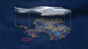
Illustration of flowing water under the Antarctic ice sheet. Blue dots indicate lakes, lines show rivers. Marie Byrd Land is part of the bulging “elbow” leading to the Antarctic Peninsula, left center. Credit: NSF/Zina Deretsky
A new NASA study adds evidence that a geothermal heat source called a mantle plume lies deep below Antarctica’s Marie Byrd Land, explaining some of the melting that creates lakes and rivers under the ice sheet. Although the heat source isn’t a new or increasing threat to the West Antarctic ice sheet, it may help explain why the ice sheet collapsed rapidly in an earlier era of rapid climate change, and why it is so unstable today.
The stability of an ice sheet is closely related to how much water lubricates it from below, allowing glaciers to slide more easily. Understanding the sources and future of the meltwater under West Antarctica is important for estimating the rate at which ice may be lost to the ocean in the future.
Antarctica’s bedrock is laced with rivers and lakes, the largest of which is the size of Lake Erie. Many lakes fill and drain rapidly, forcing the ice surface thousands of feet above them to rise and fall by as much as 20 feet (6 meters). The motion allows scientists to estimate where and how much water must exist at the base.
Some 30 years ago, a scientist at the University of Colorado Denver suggested that heat from a mantle plume under Marie Byrd Land might explain regional volcanic activity and a topographic dome feature. Very recent seismic imaging has supported this concept. When Hélène Seroussi of NASA’s Jet Propulsion Laboratory in Pasadena, California, first heard the idea, however, “I thought it was crazy,” she said. “I didn’t see how we could have that amount of heat and still have ice on top of it.”
With few direct measurements existing from under the ice, Seroussi and Erik Ivins of JPL concluded the best way to study the mantle plume idea was by numerical modeling. They used the Ice Sheet System Model (ISSM), a numerical depiction of the physics of ice sheets developed by scientists at JPL and the University of California, Irvine. Seroussi enhanced the ISSM to capture natural sources of heating and heat transport from freezing, melting and liquid water; friction; and other processes.
To assure the model was realistic, the scientists drew on observations of changes in the altitude of the ice sheet surface made by NASA’s IceSat satellite and airborne Operation IceBridge campaign. “These place a powerful constraint on allowable melt rates — the very thing we wanted to predict,” Ivins said. Since the location and size of the possible mantle plume were unknown, they tested a full range of what was physically possible for multiple parameters, producing dozens of different simulations.
They found that the flux of energy from the mantle plume must be no more than 150 milliwatts per square meter. For comparison, in U.S. regions with no volcanic activity, the heat flux from Earth’s mantle is 40 to 60 milliwatts. Under Yellowstone National Park — a well-known geothermal hot spot — the heat from below is about 200 milliwatts per square meter averaged over the entire park, though individual geothermal features such as geysers are much hotter.
Seroussi and Ivins’ simulations using a heat flow higher than 150 milliwatts per square meter showed too much melting to be compatible with the space-based data, except in one location: an area inland of the Ross Sea known for intense flows of water. This region required a heat flow of at least 150-180 milliwatts per square meter to agree with the observations. However, seismic imaging has shown that mantle heat in this region may reach the ice sheet through a rift, that is, a fracture in Earth’s crust such as appears in Africa’s Great Rift Valley.
Mantle plumes are thought to be narrow streams of hot rock rising through Earth’s mantle and spreading out like a mushroom cap under the crust. The buoyancy of the material, some of it molten, causes the crust to bulge upward. The theory of mantle plumes was proposed in the 1970s to explain geothermal activity that occurs far from the boundary of a tectonic plate, such as Hawaii and Yellowstone.
The Marie Byrd Land mantle plume formed 50 to 110 million years ago, long before the West Antarctic ice sheet came into existence. At the end of the last ice age around 11,000 years ago, the ice sheet went through a period of rapid, sustained ice loss when changes in global weather patterns and rising sea levels pushed warm water closer to the ice sheet — just as is happening today. Seroussi and Ivins suggest the mantle plume could facilitate this kind of rapid loss.
Reference:
Helene Seroussi, Erik R. Ivins, Douglas A. Wiens, Johannes Bondzio. Influence of a West Antarctic mantle plume on ice sheet basal conditions. Journal of Geophysical Research: Solid Earth, 2017; 122 (9): 7127 DOI: 10.1002/2017JB014423
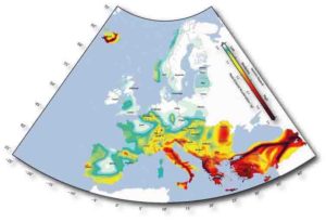
European Seismic Hazard Map. Credit: Giorgios Michas, Author provided
On September 3, 2016, a magnitude 5.8 earthquake struck just northwest of Pawnee, Oklahoma, causing moderate to severe damages in buildings near the epicenter. It was the largest ever recorded in the state.
The Pawnee earthquake followed the dramatic increase of seismic events in the central United States beginning in 2009, associated with the increase of underground wastewater disposal by oil and gas operators. This and other events in the area raised public concerns and led governmental agencies to shut down injection wells and establish new regulations regarding wastewater injections.
While human-caused earthquakes have been documented for more than a century, their increasing number reported worldwide has drawn much scientific, social and political attention. Such earthquakes are related to industrial activities such as mining, construction of water dams, injection of liquids such as waste water and carbon dioxide, and extractions associated with oil and gas exploitation.
With the ever-increasing demand for energy and mineral supplies worldwide, the number of human-caused earthquakes is expected to rise in the upcoming years. Some of the largest and more destructive earthquakes of the past few years have been related to man-made activities, such as the 2008 magnitude 7.9 Wenchuan (China) earthquake and the 2015 magnitude 7.8 Nepal earthquake.
In most of the cases industrial activities do not induce earthquakes. But this becomes problematic when such activities are close to active faults. In this case, even small stresses underground caused by man-made activities can destabilise faults, inducing earthquakes.
Faulty fluid injections
Such stresses, such as fluid injections, are even capable of migrating long distances in the planetary crust, can induce earthquakes days, months or even years after the injection.
The above figure shows that as fluid pressure at the top of the well Basel 1 (purple line) was increasing during injection, the induced seismicity rate also increased (bluish bars). In the bottom figure, the average squared distance of the induced earthquakes from the well is shown, which indicates the complex propagation of seismicity away from the well over time. The largest-earthquakes (magnitude greater than 3, shown with stars) occurred after the injection ended.
Such problems, along with the general lack of knowledge of the exact stress and faulting conditions below ground, make such earthquakes difficult to forecast or manage.
In Europe, where the population density is higher than the United States, public concern over man-made earthquakes is greater. In the well-known case of Basel, Switzerland, which took place in 2006, approximately 11,500 cubic metres of water were injected at high pressure into a 5-km deep well to make the extraction of geothermal energy possible. During the injection phase, more than 10,000 earthquakes were induced, including some strong events that were felt in Basel itself. These raised public concern and anger, leading to the termination of the project and to more than $9 million on damage claims.
Nature’s work
In Southern Europe, which has a higher risk of natural occurring earthquakes, public tolerance on induced earthquakes due to industrial activities is even more limited. The deadly 2012 Emilia (Italy) earthquake sequence became a topic of sustained public debate and political discussion, based on the proximity of the earthquake epicentres to an oil field.
The Italian government established an international committee to investigate, and while no clear link between regional seismicity and oil-extraction was found, one wasn’t excluded either. Other studies concluded that the earthquakes were a natural event.
Another recent case is that of the Castor project, an underground offshore gas-storage facility in the Gulf of Valencia, Spain. The US$2 billion project was terminated by the Spanish government in 2014 following a burst of regional seismicity immediately after the initiation of gas-injection operations, and the public concern that followed.
The above European Seismic Hazard Map displays the most seismically hazardous areas in Europe measured by the peak ground acceleration (PGA) that may be expected during an earthquake, with a 10% probability to be reached or exceeded in 50 years. Green indicates comparatively low hazard values of PGA below 0.1g; yellow to orange show a moderate hazard, between 0.1-to-0.25g; and red identify high-hazard areas with PGA of more than 0.25.
The challenges ahead
The previous cases illustrate some of the coming challenges to be faced with man-made earthquakes. The ability to distinguish between natural and human-induced earthquakes can be difficult or even impossible, especially in seismically active regions, while in other cases the risk associated with industrial activities is significantly underestimated. Such problems pose novel challenges for risk mitigation and economic growth, especially in seismically active regions such as Southern Europe.
The image above illustrates the drilling and extraction operations may take place near or within seismically active regions, increasing the risk of activating faults and/or accelerating the occurrence of earthquakes that would otherwise would occur naturally sometime in the future.
To significantly reduce such hazards, regulations are required that include hazard modelling as well as assessment before and during industrial activity that might perturb regional stress fields. Such regulations were recently issued in North America, including California, Oklahoma, Ohio and Texas, as well as in and Canada. In Europe, the EU has not yet issued any such regulations, but guidelines have been put forth in some countries that have experienced induced earthquakes, including the Netherlands, Switzerland, the UK, Germany, France and Italy.
In addition, communication campaigns that will inform the public on the economic benefits and the risks that such industrial operations may have, should also put forth. Such measures will assure the effective mitigation of the associated risk and the sustainability of the industrial project.
Mammals only started being active in the daytime after non-avian dinosaurs were wiped out about 66 million years ago (mya), finds a new study led by UCL and Tel Aviv University’s Steinhardt Museum of Natural History.
A long-standing theory holds that the common ancestor to all mammals was nocturnal, but the new discovery reveals when mammals started living in the daytime for the first time. It also provides insight into which species changed behaviour first.
The study, published today in Nature Ecology & Evolution, analysed data of 2415 species of mammals alive today using computer algorithms to reconstruct the likely activity patterns of their ancient ancestors who lived millions of years ago.
Two different mammalian family trees portraying alternative timelines for the evolution of mammals were used in the analysis. The results from both show that mammals switched to daytime activity shortly after the dinosaurs had disappeared. This change did not happen in an instant — it involved an intermediate stage of mixed day and night activity over millions of years, which coincided with the events that decimated the dinosaurs.
“We were very surprised to find such close correlation between the disappearance of dinosaurs and the beginning of daytime activity in mammals, but we found the same result unanimously using several alternative analyses,” explained lead author, PhD student Roi Maor (Tel Aviv University and UCL).
The team found that the ancestors of simian primates — such as gorillas, gibbons and tamarins — were among the first to give up nocturnal activity altogether. However, the two evolutionary timelines varied, giving a window between 52-33 mya for this to have occurred.
This discovery fits well with the fact that simian primates are the only mammals that have evolved adaptations to seeing well in daylight. The visual acuity and colour perception of simians is comparable to those of diurnal reptiles and birds — groups that never left the daytime niche.
“It’s very difficult to relate behaviour changes in mammals that lived so long ago to ecological conditions at the time, so we can’t say that the dinosaurs dying out caused mammals to start being active in the daytime. However, we see a clear correlation in our findings,” added co-author Professor Kate Jones (UCL Genetics, Evolution & Environment).
“We analysed a lot of data on the behaviour and ancestry of living animals for two reasons — firstly, because the fossil record from that era is very limited and secondly, behaviour as a trait is very hard to infer from fossils,” explained co-author, Professor Tamar Dayan (Chair of The Steinhardt Museum of Natural History, Tel Aviv University).
“You have to observe a living mammal to see if it is active at night or in the day. Fossil evidence from mammals often suggest that they were nocturnal even if they were not. Many subsequent adaptations that allow us to live in daylight are in our soft tissues.”
The team say further research is needed to better populate the mammalian family tree to give more accurate information on when the behaviour of species changes from night time to day time activity.
Reference:
Roi Maor, Tamar Dayan, Henry Ferguson-Gow, Kate E. Jones. Temporal niche expansion in mammals from a nocturnal ancestor after dinosaur extinction. Nature Ecology & Evolution, 2017; DOI: 10.1038/s41559-017-0366-5
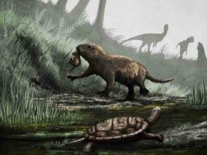
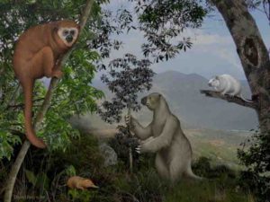
The “lost world” of Caribbean animals included ground sloths, enigmatic monkeys, giant rodents, a vampire bat, and shew-like insectivores before the arrival of humans. Credit: Illustration by D. Rini.
Although filled with tropical life today, the Caribbean islands have been a hotspot of mammal extinction since the end of the last glaciation, some 12,000 years ago. Since people also arrived after that time, it has been impossible to determine whether natural changes or human influence are most responsible for these extinctions. A new review by an international team of scientists, including Stony Brook University Professor Liliana M. Dávalos, reports an analysis of the incredibly diverse “lost world” of Caribbean fossils that includes giant rodents, vampire bats, enigmatic monkeys, ground sloths, shrews and dozens of other ancient mammals. The article, published November 6 in the Annual Review of Ecology, Evolution, and Systematics, reveals that the arrival of humans and their subsequent activities throughout the islands was likely the primary cause of the extinction of native mammal species there.
The Caribbean islands were not the only region to lose many mammal species; many large mammals from ground sloths to mastodons also vanished from continental North America. As dramatic and natural changes in the environment and the arrival of people to the continent roughly coincide in time, a scientific debate on what caused the demise of this fauna continues. Because people arrived to the islands long after the end of the glaciation, starting some 6,000 years ago, the Caribbean islands provide an ideal laboratory for discovering the cause of these losses.
In the review, the scientists report analyses of the most comprehensive radiocarbon data set of Caribbean mammals and human arrivals in the Caribbean, representing 57 extinction and extirpation (when a population vanishes from an island) events for native species. While the scattered data by themselves are invaluable, separate data points are hard to interpret, as different methods used at various sites can obscure larger patterns. So, the research team introduced a chronology developed by collecting established fossil dates reported in dozens of already-published and peer reviewed papers in an array of scientific journals.
“By using models to estimate the time of overlap between people and extinct mammals on each island, we were able to show most mammal extinctions happened after the arrival of humans on various islands in the Caribbean, and not before,” explained Dávalos, who led the quantitative analyses of the study. While the overlap between people and the fauna is not proof positive of human causes for the many extinction events in the region, it is an important step to determine why these mammals went extinct. Weaving together data from the many journal articles and archaeological site reports, the team concluded that the timing of extinctions indicates humans may be involved in the extinction of more than 60% of the nearly 150 native mammal species.
Multiple waves of human settlement in the Caribbean occurred over the past six to seven thousand years. The first settlers, Amerindian people from South or Central America known as the Lithic culture, were followed by two other waves — the Archaic and Ceramic, both from South America. The authors showed that after the initial waves of human arrival, mammal extinctions followed, presumably first caused by hunting and later by forest clearing for agriculture, which reduces the habitat for native mammals. A final wave of human migration, this time from across the Atlantic, brought with it cats, rats, goats, mongoose, and other introduced mammals. The ensuing change in habitats, and both competition and predation, resulted in the extinction of about a dozen populations on the smaller islands of the Lesser Antilles. These predators and competitors can affect the populations of Caribbean mammals that survived previous extinction waves.
“While this article is the result of an important collaboration of scientists — with each author bringing their expertise to the table to solve the puzzle mammal extinction — saving the community of mammals of today needs a much wider group of professionals, especially on each island, which is why we are assembling a larger team,” she added.
Dávalos’ team is now working to bring together a larger, interdisciplinary team of colleagues to create an intensive conservation management plan incorporating the expertise of conservation researchers, biologist, ecologists, policy-makers, educators, and land and wildlife management experts to save the last surviving native Caribbean mammals.
“In examining data from both paleontological digs and archeological reports, the evidence highlights the need for urgent human intervention to protect the native mammal species still inhabiting the region, and that is why we are coming together with scientists from all over the Caribbean,” concluded Dávalos.
Reference:
Siobhán B. Cooke, Liliana M. Dávalos, Alexis M. Mychajliw, Samuel T. Turvey, Nathan S. Upham. Anthropogenic Extinction Dominates Holocene Declines of West Indian Mammals. Annual Review of Ecology, Evolution, and Systematics, 2016; 48 (1) DOI: 10.1146/annurev-ecolsys-110316-022754
Artist’s conception of comet approaching Earth-like planet. The explosion of a comet near our planet’s surface, it was proposed, might have lofted enough dust and debris into Earth’s atmosphere to temporarily dim the sun. Credit: Shutterstock
Chemists at The Scripps Research Institute (TSRI) have found a compound that may have been a crucial factor in the origins of life on Earth.
Origins-of-life researchers have hypothesized that a chemical reaction called phosphorylation may have been crucial for the assembly of three key ingredients in early life forms: short strands of nucleotides to store genetic information, short chains of amino acids (peptides) to do the main work of cells, and lipids to form encapsulating structures such as cell walls. Yet, no one has ever found a phosphorylating agent that was plausibly present on early Earth and could have produced these three classes of molecules side-by-side under the same realistic conditions.
TSRI chemists have now identified just such a compound: diamidophosphate (DAP).
“We suggest a phosphorylation chemistry that could have given rise, all in the same place, to oligonucleotides, oligopeptides, and the cell-like structures to enclose them,” said study senior author Ramanarayanan Krishnamurthy, associate professor of chemistry at TSRI. “That in turn would have allowed other chemistries that were not possible before, potentially leading to the first simple, cell-based living entities.”
The study, reported in Nature Chemistry, is part of an ongoing effort by scientists around the world to find plausible routes for the epic journey from pre-biological chemistry to cell-based biochemistry.
Other researchers have described chemical reactions that might have enabled the phosphorylation of pre-biological molecules on the early Earth. But these scenarios have involved different phosphorylating agents for different types of molecule, as well as different and often uncommon reaction environments.
“It has been hard to imagine how these very different processes could have combined in the same place to yield the first primitive life forms,” said Krishnamurthy.
He and his team, including co-first authors Clémentine Gibard, Subhendu Bhowmik, and Megha Karki, all postdoctoral research associates at TSRI, showed first that DAP could phosphorylate each of the four nucleoside building blocks of RNA in water or a paste-like state under a wide range of temperatures and other conditions.
With the addition of the catalyst imidazole, a simple organic compound that was itself plausibly present on the early Earth, DAP’s activity also led to the appearance of short, RNA-like chains of these phosphorylated building blocks.
Moreover, DAP with water and imidazole efficiently phosphorylated the lipid building blocks glycerol and fatty acids, leading to the self-assembly of small phospho-lipid capsules called vesicles — primitive versions of cells.
DAP in water at room temperature also phosphorylated the amino acids glycine, aspartic acid and glutamic acid, and then helped link these molecules into short peptide chains (peptides are smaller versions of proteins).
“With DAP and water and these mild conditions, you can get these three important classes of pre-biological molecules to come together and be transformed, creating the opportunity for them to interact together,” Krishnamurthy said.
Krishnamurthy and his colleagues have shown previously that DAP can efficiently phosphorylate a variety of simple sugars and thus help construct phosphorus-containing carbohydrates that would have been involved in early life forms. Their new work suggests that DAP could have had a much more central role in the origins of life.
“It reminds me of the Fairy Godmother in Cinderella, who waves a wand and ‘poof,’ ‘poof,’ ‘poof,’ everything simple is transformed into something more complex and interesting,” Krishnamurthy said.
DAP’s importance in kick-starting life on Earth could be hard to prove several billion years after the fact. Krishnamurthy noted, though, that key aspects of the molecule’s chemistry are still found in modern biology.
“DAP phosphorylates via the same phosphorus-nitrogen bond breakage and under the same conditions as protein kinases, which are ubiquitous in present-day life forms,” he said. “DAP’s phosphorylation chemistry also closely resembles what is seen in the reactions at the heart of every cell’s metabolic cycle.”
Krishnamurthy now plans to follow these leads, and he has also teamed with early-Earth geochemists to try to identify potential sources of DAP, or similarly acting phosphorus-nitrogen compounds, that were on the planet before life arose.
“There may have been minerals on the early Earth that released such phosphorus-nitrogen compounds under the right conditions,” he said. “Astronomers have found evidence for phosphorus-nitrogen compounds in the gas and dust of interstellar space, so it’s certainly plausible that such compounds were present on the early Earth and played a role in the emergence of the complex molecules of life.”
Reference:
Clémentine Gibard, Subhendu Bhowmik, Megha Karki, Eun-Kyong Kim, Ramanarayanan Krishnamurthy. Phosphorylation, oligomerization and self-assembly in water under potential prebiotic conditions. Nature Chemistry, 2017; DOI: 10.1038/nchem.2878
A new study looks at rock from the titanic eruption that formed Long Valley Caldera in California 765,000 years ago. Calderas occur when a volcano collapses after an eruption. Long Valley has been studied by Wes Hildreth (in background), an author of the new PNAS study, for decades. The study signals that we don’t fully understand these giant eruptions. Credit: U.S. Geological Survey
Long Valley, California, has long defined the “super-eruption.” About 765,000 years ago, a pool of molten rock exploded into the sky. Within one nightmarish week, 760 cubic kilometers of lava and ash spewed out in the kind of volcanic cataclysm we hope never to witness.
The ash likely cooled the planet by shielding the sun, before settling across the western half of North America.
Here’s a rule of geoscience: The past heralds the future. So it’s not just morbid curiosity that attracts geoscientists to places like Long Valley. It’s an ardent desire to understand why super-eruptions happen, ultimately to understand where and when they are likely to occur again.
This week (Nov. 6, 2017), in the Proceedings of the National Academy of Sciences, a report shows that the giant body of magma—molten rock—at Long Valley was much cooler before the eruption than previously thought.
“The older view is that there’s a long period with a big tank of molten rock in the crust,” says first author Nathan Andersen, who recently graduated from the University of Wisconsin-Madison with a Ph.D. in geoscience. “But that idea is falling out of favor.
“A new view is that magma is stored for a long period in a state that is locked, cool, crystalline, and unable to produce an eruption. That dormant system would need a huge infusion of heat to erupt.”
It’s hard to understand how the rock could be heated from an estimated 400 degrees Celsius to the 700 to 850 degrees needed to erupt, but the main cause must be a quick rise of much hotter rock from deep below.
Instead of a long-lasting pool of molten rock, the crystals from solidified rock were incorporated shortly before the eruption, Andersen says. So the molten conditions likely lasted only a few decades, at most a few centuries. “Basically, the picture has evolved from the ‘big tank’ view to the ‘mush’ view, and now we propose that there is an underappreciation of the contribution of the truly cold, solidified rock.”
The new results are rooted in a detailed analysis of argon isotopes in crystals from the Bishop Tuff—the high-volume rock released when the Long Valley Caldera formed. Argon, produced by the radioactive decay of potassium, quickly escapes from hot crystals, so if the magma body that contained these crystals was uniformly hot before eruption, argon would not accumulate, and the dates for all 49 crystals should be the same.
And yet, using a new, high-precision mass spectrometer in the Geochronology Lab at UW-Madison, the research group’s dates spanned a 16,000 year range, indicating the presence of some argon that formed long before the eruption. That points to unexpectedly cool conditions before the giant eruption.
Better tools make better science, Andersen says. “The new instrument is more sensitive than its predecessors, so it can measure a smaller volume of gas with higher precision. When we looked in greater detail at single crystals, it became clear some must have been derived from magma that had completely solidified—transitioned from a mush to a rock.”
“Nathan found that about half of the crystals began to crystallize a few thousand years before the eruption, indicating cooler conditions,” says Brad Singer, a professor of geoscience at UW-Madison and director of the Geochronology Lab. “To get the true eruption age, you need to see the dispersion of dates. The youngest crystals show the date of eruption.”
The results have meaning beyond volcanology, however, as ash from Long Valley and other giant eruptions is commonly used for dating.
“These huge eruptions deposit ash all over the place, and that lets you make correlations in the rock record to aid geologic, biologic and climatic studies across the continent,” says Andersen. “This blanket of ash anchors you in time. The closer we can pin down the eruption age, the better we can study all facets of Earth’s history.”
“It’s controversial, but finding these older crystals means that part of this large magma body was very cool immediately prior to eruption,” says Singer, a volcanologist who was Andersen’s UW advisor. “This flies in the face of a lot of thermodynamics.”
A better understanding of the pre-eruption process could lead to better volcano forecasting—a highly useful but difficult proposition at present.
“This does not point to prediction in any concrete way,” says Singer, “but it does point to the fact that we don’t understand what is going on in these systems, in the period of 10 to 1,000 years that precedes a large eruption.”
Reference:
Nathan L. Andersen el al., “Incremental heating of Bishop Tuff sanidine reveals preeruptive radiogenic Ar and rapid remobilization from cold storage,” PNAS (2017). DOI: 10.1073/pnas.1709581114
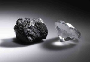
A new study by Washington State University researchers answers longstanding questions about the formation of a rare type of diamond during major meteorite strikes.
Hexagonal diamond or lonsdaleite is harder than the type of diamond typically worn on an engagement ring and is thought to be naturally made when large, graphite-bearing meteorites slam into Earth.
Scientists have puzzled over the exact pressure and other conditions needed to make hexagonal diamond since its discovery in an Arizona meteorite fragment half a century ago.
Now, a team of WSU researchers has for the first time observed and recorded the creation of hexagonal diamond in highly oriented pyrolytic graphite under shock compression, revealing crucial details about how it is formed. The discovery could help planetary scientists use the presence of hexagonal diamond at meteorite craters to estimate the severity of impacts.
The research was possible because of an unprecedented experimental development-the WSU-led Dynamic Compression Sector at Argonne National Laboratory’s Advanced Photon Source. The DCS is a first-of-its-kind experimental facility that links different shock wave compression capabilities to synchrotron x-rays. Using its unique capabilities, the WSU team was able to take x-ray snap shots of the transformation of graphite to hexagonal diamond in real-time.
The results of the researchers’ work are published in the journal Science Advances.
“The transformation to hexagonal diamond occurs at a significantly lower stress than previously believed,” said WSU Regents Professor Yogendra Gupta, director of the Institute for Shock Physics and a co-author of the study. “This result has important implications regarding the estimates of thermodynamic conditions at the terrestrial sites of meteor impacts.”
Making diamonds
WSU shock physicist Stefan Turneaure and a team of researchers found that the crystalline structure of a highly oriented form of graphite transforms to the uncommon hexagonal form of diamond at a pressure of 500,000 atmospheres, around four times lower than previous studies had indicated.
To obtain their results, the researchers shot a lithium fluoride impactor at 11,000 mph into a 2 mm thick graphite disk. They then used pulsed synchrotron x-rays to take snapshots every 150 billionths of a second while the shockwave from the impact compressed the graphite sample. Their work clearly showed the graphite sample transformed into the hexagonal form of diamond before being obliterated into dust.
“Most past research relied on microstructural examination of samples after they were shock compressed to infer what might have happened,” Turneaure said. “Such late-time measurements do not tell the whole story of what happened to the material during shock compression.”
Moving forward
Turneaure and Gupta said the next step in the research will be to investigate under what conditions pure hexagonal diamond can be recovered after shock compression.
“Diamond is a material that is very easy to get excited about and our work in this area is just beginning,” Gupta said. “Moving forward, we plan to investigate the persistence of this form of diamond under lower pressure. Because it is thought to be 60 percent harder than the common cubic diamond, hexagonal diamond could have many potential uses in industry if it could be successfully recovered after shock compression.”
Reference:
Transformation of shock-compressed graphite to hexagonal diamond in nanoseconds. DOI: 10.1126/sciadv.aao3561
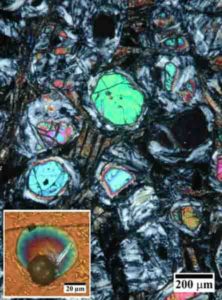
Photomicrographs of fresh olivine (large green, blue and pink crystals) and glass inclusion (lower left inset). Komatiite volcanic rocks from the 3.3 billion-year-old Weltevreden Formation are the freshest yet discovered in from Earth’s early Archean. Trace elements, radiogenic and stable isotopes from these rocks and olivine separates provide key evidence for evolution of Earth’s mantle. Credit: Keena Kareem, LSU
The first 1.5 billion years of Earth’s evolution is subject to considerable uncertainty due to the lack of any significant rock record prior to four billion years ago and a very limited record until about three billion years ago. Rocks of this age are usually extensively altered making comparisons to modern rock quite difficult. In new research conducted at LSU, scientists have found evidence showing that komatiites, three-billion-year old volcanic rock found within the Earth’s mantle, had a different composition than modern ones. Their discovery may offer new information about the first one billion years of Earth’s development and early origins of life. Results of the team’s work has been published in the October 2017 edition of NATURE Geoscience.
The basic research came from more than three decades of LSU scientists studying and mapping the Barberton Mountains of South Africa. The research team, including LSU geology professors Gary Byerly and Huiming Bao, geology PhD graduate Keena Kareem, and LSU researcher Benjamin Byerly, conducted chemical analyses of hundreds of komatiite rocks sampled from about 10 lava flows.
“Early workers had mapped large areas incorrectly by assuming they were correlatives to the much more famous Komati Formation in the southern part of the mountains. We recognized this error and began a detailed study of the rocks to prove our mapping-based interpretations,” said Gary Byerly.
Within the rocks, they discovered original minerals called fresh olivine, which had been preserved in remarkable detail. Though the mineral is rarely found in rocks subjected to metamorphism and surface weathering, olivine is the major constituent of Earth’s upper mantle and controls the nature of volcanism and tectonism of the planet. Using compositions of these fresh minerals, the researchers had previously concluded that these were the hottest lavas to ever erupt on Earth’s surface with temperatures near 1600 degrees centigrade, which is roughly 400 degrees hotter than modern eruptions in Hawaii.
“Discovering fresh unaltered olivine in these ancient lavas was a remarkable find. The field work was wonderfully productive and we were eager to return to the lab to use the chemistry of these preserved olivine crystals to reveal clues of the Archean Mantle,” said Kareem
The researchers suggest that maybe a chunk of early-Earth magma ocean is preserved in the approximately 3.2 billion year-old minerals.
“The modern Earth shows little or no evidence of this early magma ocean because convection of the mantle has largely homogenized the layering produced in the magma ocean. Oxygen isotopes in these fresh olivines support the existence of ancient chunks of the frozen magma ocean. Rocks like this are very rare and scientifically valuable. An obvious next step was to do oxygen isotopes,” said Byerly.
This study grew out of work taking place in LSU’s laboratory for the study of oxygen isotopes, a world-class facility that attracts scientists from the U.S. and international institutions for collaborative work. The results of the study were so unusual that it required extra care to be certain of the results. Huiming Bao, who is also the head of LSU’s oxygen isotopes lab, said that the team triple and quadruple checked the data by running with different reference minerals and by calibrating with other independent labs.
“We attempted to reconcile the findings with some of the conventional explanations for lavas with oxygen isotope compositions like these, but nothing could fully explain all of the observations. It became apparent that these rocks preserve signatures of processes that occurred over four billion years ago and that are still not completely understood,” said Benjamin Byerly.
Oxygen isotopes are measured by the conversion of rock or minerals into a gas and measuring the ratios of oxygen with the different masses of 16, 17, and 18. A variety of processes fractionate oxygen on Earth and in the Solar System, including atmospheric, hydrospheric, biological, and high temperature and pressure.
“Different planets in our solar system have different oxygen isotope ratios. On Earth this is modified by surface atmosphere and hydrosphere, so variations could be due either to heterogeneous mantle (original accumulation of planetary debris or remnants of magma ocean) or surface processes,” said Byerly. “Either might be interesting to study. The latter because it would also provide information about the early surface temperature of Earth and early origins of life.”
This work was supported by a National Science Foundation grant awarded to Byerly, a NASA grant awarded to Bao, and general support from LSU.
Reference:
Benjamin L. Byerly, Keena Kareem, Huiming Bao, Gary R. Byerly. Early Earth mantle heterogeneity revealed by light oxygen isotopes of Archaean komatiites. Nature Geoscience, 2017; 10 (11): 871 DOI: 10.1038/ngeo3054
A mammoth tusk on Wrangel Island. Credit: Patrícia Pe?nerová
Researchers who have sexed 98 woolly mammoth specimens collected from various parts of Siberia have discovered that the fossilized remains more often came from males of the species than females. They speculate that this skewed sex ratio — seven out of every ten specimens examined belonged to males — exists in the fossil record because inexperienced male mammoths more often travelled alone and got themselves killed by falling into natural traps that made their preservation more likely. The findings are reported in Current Biology on November 2.
“Most bones, tusks, and teeth from mammoths and other Ice Age animals haven’t survived,” said Love Dalen of the Swedish Museum of Natural History. “It is highly likely that the remains that are found in Siberia these days have been preserved because they have been buried, and thus protected from weathering. The new findings imply that male mammoths more often died in a way that meant their remains were buried, perhaps by falling through lake ice in winter or getting stuck in bogs.”
“We were very surprised because there was no reason to expect a sex bias in the fossil record,” added Patrícia Pecnerova, the study’s first author, also at the Swedish Museum of Natural History. “Since the ratio of females to males was likely balanced at birth, we had to consider explanations that involved better preservation of male remains.”
The researchers made the discovery in the midst of a larger, long-term effort to examine the genomes of woolly mammoth populations. For some of the analyses, they needed to know the sex of individuals. They initially set out to determine the sex of a small number of mammoths. “It became apparent that we were finding an excess of male samples, which we found very interesting,” Dalen said.
They decided to sex more samples and to examine the sex ratio of individuals collected from the Siberian mainland and from Wrangel Island, off the coast. Overall, they found, males consistently outnumbered females among their samples.
The researchers say the findings suggest that woolly mammoths lived similarly to modern elephants, with herds of females and young elephants led by an experienced adult female. In contrast, they suspect that male mammoths, like elephants, more often lived in bachelor groups or alone and engaged in more risk-taking behavior.
“Without the benefit of living in a herd led by an experienced female, male mammoths may have had a higher risk of dying in natural traps such as bogs, crevices, and lakes,” Dalen said.
The findings highlight the utility of fossil remains for making inferences about the socioecology and behavior of extinct animals, the researchers say. At the same time, they are a reminder to researchers that fossil assemblages don’t necessarily represent a random sample of a population.
The researchers say they’ll continue to study woolly mammoth genomes and those of several other extinct Ice Age mammals. They’re curious to see whether they observe the same skewed sex ratio in other species.
Reference:
Pecnerova et al. Genome-Based Sexing Provides Clues about Behavior and Social Structure in the Woolly Mammoth. Current Biology, 2017 DOI: 10.1016/j.cub.2017.09.064
Note: The above post is reprinted from materials provided by Cell Press.
Foraminifera Orbulina Universa eating a small copepod. Credit: Oscar Branson/ANU
The results of new international research into tiny marine plankton will allow scientists to more precisely estimate past ocean conditions and predict future changes, and suggests global warming may have a bigger impact on shell-bearing plankton than previously thought.
Tiny marine plankton, foraminifers, record information about the environment in which they grew in the chemical composition of their carbonate shells. Foraminifer shells are one of our most important climate archives. Reading these archives correctly is key to understand past and to predict future climate.
Researchers from Macquarie University, the GFZ German Research Centre for Geosciences in Potsdam and The Australian National University have used transmission electron microscopy to examine ultra-thin slices of these shells, to understand how the shells record ocean conditions.
“Magnesium found in the plankton shells, for example, is used to calculate seawater temperatures going back tens of millions of years,” said lead researcher Professor Dorrit Jacob, of Macquarie University’s Department of Earth and Planetary Sciences.
“Understanding how the shells develop is key to understanding how magnesium and other elements get into the shells, and therefore how we read the shells’ climate records.”
As published in Nature Communications, the team found these plankton shells first form as the unstable carbonate vaterite, which eventually transforms into stable calcite.
“This was a big surprise. Since the 1950s, we’ve thought the shells were made directly of calcite – and this is what we have been teaching students to this day,” stated Dr. Jacob.
“Which type of carbonate forms first, vaterite or calcite, determines how much magnesium is incorporated into the shell. This finding about how foraminifer shells form will now enable us to estimate past ocean temperatures more precisely, and more accurately predict future climate change.”
The presence of unstable vaterite in these abundant organisms also means foraminifer shells may be far more susceptible to ocean acidification than previously thought. This could have drastic ramifications for carbon dioxide transfer to the deep ocean and seafloor in the marine carbon cycle, as foraminifer shells are dense and assist rapid sinking of organic matter.
Reference:
D. E. Jacob et al, Planktic foraminifera form their shells via metastable carbonate phases, Nature Communications (2017). DOI: 10.1038/s41467-017-00955-0
Note: The above post is reprinted from materials provided by Macquarie University.
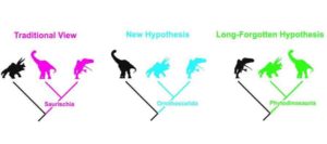
Two possible branches of the dinosaur family tree (left and middle). Credit: Max Langer
The classification of the dinosaurs might seem to be too obscure to excite anyone but the specialists.
However, this is not at all the case. Recently, Matthew Baron and colleagues from the University of Cambridge proposed a radical revision to our understanding of the major branches of dinosaurs, but in a critique published today some caution is proposed before we rewrite the textbooks.
Every child learns that dinosaurs fall into two major groups, the Ornithischia (bird-hipped dinosaurs; Stegosaurus, Triceratops, Iguanodon and their kin) and the Saurischia (lizard-hipped dinosaurs; the predatory theropods, such as Tyrannosaurus, and the long-necked sauropodomorphs, including such well-known forms as Diplodocus).
Baron and colleagues proposed a very different split, pairing the Ornithischia with the Theropoda, terming the new group the Ornithoscelida, and leaving the Sauropodomorpha on its own.
Their evidence seemed overwhelming, since they identified at least 18 unique characters shared by ornithischians and theropods, and used these as evidence that the two groups had shared a common ancestor.
An international consortium of specialists in early dinosaurs, led by Max Langer from the Universidade de São Paulo, Brazil, and including experts from Argentina, Brazil, Germany, Great Britain, and Spain has now re-evaluated the data provided by Baron et al. in support of their claim.
Their results, presented today in the journal Nature, show that it might still be too early to re-write the textbooks for dinosaurs.
In this new evaluation, the authors found support for the traditional model of an Ornithischia-Saurischia split of Dinosauria, but also noted that this support was very weak, and the alternative idea of Ornithoscelida is only slightly less likely.
Max Langer said: “This took a great deal of work by our consortium, checking many dinosaurs on all continents first-hand to make sure we coded their characters correctly.
“We thought at the start we might only cast some doubt on the idea of Ornithoscelida, but I’d say the whole question now has to be looked at again very carefully.”
Baron and colleagues believed their data suggested that dinosaurs might have originated in the northern hemisphere, but the re-analysis confirms the long-held view that the most likely site of origin is the southern hemisphere, and probably South America.
Professor Mike Benton from the University of Bristol’s School of Earth Sciences, a member of the revising consortium, added: “In science, if you wish to overthrow the standard viewpoint, you need strong evidence.
“We found the evidence to be pretty balanced in favour of two possible arrangements at the base of the dinosaurian tree. Baron and colleagues might be correct, but we would argue that we should stick to the orthodox Saurischia-Ornithischia split for the moment until more convincing evidence emerges.”
Steve Brusatte of the University of Edinburgh, a member of the consortium, said: “Up until this year, we thought we had the dinosaur family tree figured out.
“But right now, we just can’t be certain how the three major groups of dinosaurs are related to each other. In one sense it’s frustrating, but in another, it’s exciting because it means that we need to keep finding new fossils to solve this mystery.”
Reference:
Max C. Langer, Martín D. Ezcurra, Oliver W. M. Rauhut, Michael J. Benton, Fabien Knoll, Blair W. McPhee, Fernando E. Novas, Diego Pol, Stephen L. Brusatte. Untangling the dinosaur family tree. Nature, 2017; 551 (7678): E1 DOI: 10.1038/nature24011
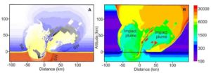
A simulation of the crater and impact plume formed eight seconds after the Chicxulub impact at 45 degrees. Chart A shows the density of different materials created in the impact. The colors show the atmosphere (blue), sediment (yellow), asteroid (gray) and basement (red), with darker colors reflecting higher densities. SW is the shock wave formed by the impact. Chart B shows the temperature in Kelvin at different locations in the impact. Credit: Pierazzo and Artemieva (2012).
The Chicxulub asteroid impact that wiped out the dinosaurs likely released far more climate-altering sulfur gas into the atmosphere than originally thought, according to new research.
A new study makes a more refined estimate of how much sulfur and carbon dioxide gas were ejected into Earth’s atmosphere from vaporized rocks immediately after the Chicxulub event. The study’s authors estimate more than three times as much sulfur may have entered the air compared to what previous models assumed, implying the ensuing period of cool weather may have been colder than previously thought.
The new study lends support to the hypothesis that the impact played a significant role in the Cretaceous–Paleogene extinction event that eradicated nearly three-quarters of Earth’s plant and animal species, according to Joanna Morgan, a geophysicist at Imperial College London in the United Kingdom and co-author of the new study published in Geophysical Research Letters, a journal of the American Geophysical Union.
“Many climate models can’t currently capture all of the consequences of the Chicxulub impact due to uncertainty in how much gas was initially released,” Morgan said. “We wanted to revisit this significant event and refine our collision model to better capture its immediate effects on the atmosphere.”
The new findings could ultimately help scientists better understand how Earth’s climate radically changed in the aftermath of the asteroid collision, according to Georg Feulner, a climate scientist at the Potsdam Institute for Climate Impact Research in Potsdam, Germany who was not involved with the new research. The research could help give new insights into how Earth’s climate and ecosystem can significantly change due to impact events, he said.
“The key finding of the study is that they get a larger amount of sulfur and a smaller amount of carbon dioxide ejected than in other studies,” he said. “These improved estimates have big implications for the climactic consequences of the impact, which could have been even more dramatic than what previous studies have found.”
A titanic collision
The Chicxulub impact occurred 66 million years ago when an asteroid approximately 12 kilometers (7 miles) wide slammed into Earth. The collision took place near what is now the Yucatán peninsula in the Gulf of Mexico. The asteroid is often cited as a potential cause of the Cretaceous-Paleogene extinction event, a mass extinction that erased up to 75 percent of all plant and animal species, including the dinosaurs.
The asteroid collision had global consequences because it threw massive amounts of dust, sulfur and carbon dioxide into the atmosphere. The dust and sulfur formed a cloud that reflected sunlight and dramatically reduced Earth’s temperature. Based on earlier estimates of the amount of sulfur and carbon dioxide released by the impact, a recent study published in Geophysical Research Letters showed Earth’s average surface air temperature may have dropped by as much as 26 degrees Celsius (47 degrees Fahrenheit) and that sub-freezing temperatures persisted for at least three years after the impact.
In the new research, the authors used a computer code that simulates the pressure of the shock waves created by the impact to estimate the amounts of gases released in different impact scenarios. They changed variables such as the angle of the impact and the composition of the vaporized rocks to reduce the uncertainty of their calculations.
The new results show the impact likely released approximately 325 gigatons of sulfur and 425 gigatons of carbon dioxide into the atmosphere, more than 10 times global human emissions of carbon dioxide in 2014. In contrast, the previous study in Geophysical Research Letters that modeled Earth’s climate after the collision had assumed 100 gigatons of sulfur and 1,400 gigatons of carbon dioxide were ejected as a result of the impact.
Improving the impact model
The new study’s methods stand out because they ensured only gases that were ejected upwards with a minimum velocity of 1 kilometer per second (2,200 miles per hour) were included in the calculations. Gases ejected at slower speeds didn’t reach a high enough altitude to stay in the atmosphere and influence the climate, according to Natalia Artemieva, a senior scientist at the Planetary Science Institute in Tucson, Arizona and co-author of the new study.
Older models of the impact didn’t have as much computing power and were forced to assume all the ejected gas entered the atmosphere, limiting their accuracy, Artemieva said.
The study authors also based their model on updated estimates of the impact’s angle. An older study assumed the asteroid hit the surface at an angle of 90 degrees, but newer research shows the asteroid hit at an angle of approximately 60 degrees. Using this revised angle of impact led to a larger amount of sulfur being ejected into the atmosphere, Morgan said.
The study’s authors did not model how much cooler Earth would have been as a result of their revised estimates of how much gas was ejected. Judging from the cooling seen in the previous study, which assumed a smaller amount of sulfur was released by the impact, the release of so much sulfur gas likely played a key role in the extinction event. The sulfur gas would have blocked out a significant amount of sunlight, likely leading to years of extremely cold weather potentially colder than the previous study found. The lack of sunlight and changes in ocean circulation would have devastated Earth’s plant life and marine biosphere, according to Feulner.
The release of carbon dioxide likely led to some long-term climate warming, but its influence was minor compared to the cooling effect of the sulfur cloud, Feulner said.
Along with gaining a better understand of the Chicxulub impact, researchers can also use the new study’s methods to estimate the amount of gas released during other large impacts in Earth’s history. For example, the authors calculated the Ries crater located in Bavaria, Germany was formed by an impact that ejected 1.3 gigatons of carbon dioxide into the atmosphere. This amount of gas likely had little effect on Earth’s climate, but the idea could be applied to help understand the climactic effects of larger impacts.
Reference:
Natalia Artemieva, Joanna Morgan. Quantifying the Release of Climate-Active Gases by Large Meteorite Impacts With a Case Study of Chicxulub. Geophysical Research Letters, 2017; DOI: 10.1002/2017GL074879
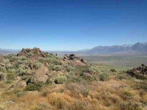
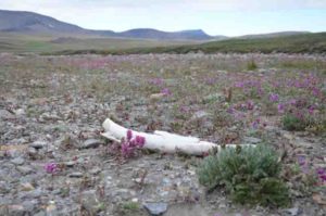
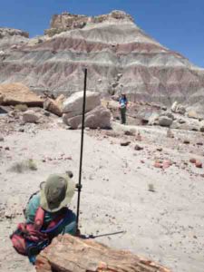
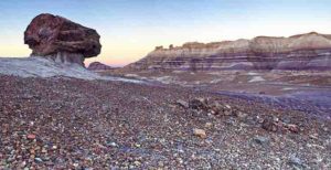
URI junior Amanda Bednarick (background) and research assistant Sam Hemmendinger use a Jacob’s staff to measure the thickness of rocks at Petrified Forest National Park. Credit: Reilly Hayes
One of the most exciting discoveries that paleontologists can make is finding the causal relationship between the extinction of ancient creatures and the environmental conditions that led to that extinction. A team of scientists and students at the University of Rhode Island is inching closer to revealing how a group of animals from the Late Triassic went extinct, thanks to the precise dating of fossils at Petrified Forest National Park in Arizona.
URI Professor David Fastovsky, who made important discoveries about the extinction of the dinosaurs between the Cretaceous and Tertiary periods 66 million years ago, is leading a team of researchers working to understand what caused the extinction of the near-relatives of North America’s earliest dinosaurs around 215 million years ago.
“Reconstructing extinctions is extremely difficult,” he said, “but at Petrified Forest we have the best-dated ancient river deposits in the world, which allow us to ask very precise questions about this extinction — in particular, whether it was gradual or catastrophic. This could be one of the extremely rare instances in the ancient record when this could actually be determined quantitatively using direct evidence.”
If the researchers determine that all of the animals went extinct at about the same time — rather than gradually over a long period — they may be able to link the animals’ extinction to the catastrophic impact of an asteroid that left a 50-mile-wide crater in Quebec, an impact that some scientists believe was responsible for the extinctions at that time.
Fastovsky has been studying the fossils at Petrified Forest since 1991. He said the rocks there indicate a distinct “faunal turnover” when one set of organisms disappeared and another set of organisms appeared.
“The question is, can we date that faunal turnover, and how precisely,” he said.
Using what he called “high-precision uranium-lead dating” developed by researchers at the Massachusetts Institute of Technology and applied by URI geoscientists in Petrified Forest National Park, Fastovsky is hopeful that his team will have some answers by the end of next year.
To meet that goal, Fastovsky engaged Gavino Puggioni, URI assistant professor of statistics, who is using sophisticated statistical analyses to determine whether the ancient animals all went extinct simultaneously, which would be expected from a catastrophic event.
“The processes that we’re studying took place over thousands of years,” said Puggioni. “We’re trying to extract a very weak signal from this small data set. But there are statistical techniques that can help us identify what we’re observing. We are trying to extend and push the boundaries.”
“This is an unheard-of level of quantitative precision being applied to an extinction event,” added Fastovsky.
To fill in gaps in the existing data, URI graduate student Reilly Hayes and junior Amanda Bednarick spent three months last summer finding the precise locations where more than 100 fossils had been collected from Petrified Forest over the last century. It wasn’t easy.
“River systems like at Petrified Forest tear themselves up when the sediments build up,” explained Hayes. “So you find a lot of discontinuities between the beds of rock. But we already had dates in the model of how certain beds fit together into the larger sequence at the park. We just didn’t know where all the fossils occurred relative to those.”
The dates in the model were first collected by a previous generation of URI researchers, and they run through the full thickness of the rock sequence exposed in the Park, which Fastovsky and his MIT colleagues nicknamed the “backbone.”
Hayes and Bednarick hiked many miles each week last summer and found 51 sites around the park where they could link previously collected fossils with rocks of known age.
“We relocated all these fossil localities, some of which didn’t have exact information for where they were originally found, and then we established a game plan for how to correlate this spot on the ground to a place where the backbone was exposed,” said Bednarick.
Over the next year, additional field work will be required to relocate about 20 more fossil sites, and the statistical analyses will continue. And then the researchers hope to be able to draw conclusions about the cause of the extinction.
“We’re looking forward to testing whether the extinctions occurred at the same time and whether this particular extinction would be concordant with what you would expect if an asteroid did the deed,” concluded Fastovsky. “That would be pretty special.”
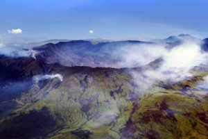
An aerial view of Mount Tambora’s caldera, formed during the 1815 eruption. Credit: Wikipedia
Major volcanic eruptions in the future have the potential to affect global temperatures and precipitation more dramatically than in the past because of climate change, according to a new study led by the National Center for Atmospheric Research (NCAR).
The study authors focused on the cataclysmic eruption of Indonesia’s Mount Tambora in April 1815, which is thought to have triggered the so-called “year without a summer” in 1816. They found that if a similar eruption occurred in the year 2085, temperatures would plunge more deeply, although not enough to offset the future warming associated with climate change. The increased cooling after a future eruption would also disrupt the water cycle more severely, decreasing the amount of precipitation that falls globally.
The reason for the difference in climate response between 1815 and 2085 is tied to the oceans, which are expected to become more stratified as the planet warms, and therefore less able to moderate the climate impacts caused by volcanic eruptions.
“We discovered that the oceans play a very large role in moderating, while also lengthening, the surface cooling induced by the 1815 eruption,” said NCAR scientist John Fasullo, lead author of the new study. “The volcanic kick is just that — it’s a cooling kick that lasts for a year or so. But the oceans change the timescale. They act to not only dampen the initial cooling but also to spread it out over several years.”
The research will be published Oct. 31 in the journal Nature Communications. The work was funded in part by the National Science Foundation, NCAR’s sponsor. Other funders include NASA and the U.S. Department of Energy. The study co-authors are Robert Tomas, Samantha Stevenson, Bette Otto-Bliesner, and Esther Brady, all of NCAR, as well as Eugene Wahl, of the National Oceanic and Atmospheric Administration.
A detailed look at a deadly past
Mount Tambora’s eruption, the largest in the past several centuries, spewed a huge amount of sulfur dioxide into the upper atmosphere, where it turned into sulfate particles called aerosols. The layer of light-reflecting aerosols cooled Earth, setting in motion a chain of reactions that led to an extremely cold summer in 1816, especially across Europe and the northeast of North America. The “year without a summer” is blamed for widespread crop failure and disease, causing more than 100,000 deaths globally.
To better understand and quantify the climate effects of Mount Tambora’s eruption, and to explore how those effects might differ for a future eruption if climate change continues on its current trajectory, the research team turned to a sophisticated computer model developed by scientists from NCAR and the broader community.
The scientists looked at two sets of simulations from the Community Earth System Model. The first was taken from the CESM Last Millennium Ensemble Project, which simulates Earth’s climate from the year 850 through 2005, including volcanic eruptions in the historic record. The second set, which assumes that greenhouse gas emission continue unabated, was created by running CESM forward and repeating a hypothetical Mount Tambora eruption in 2085.
The historical model simulations revealed that two countervailing processes helped regulate Earth’s temperature after Tambora’s eruption. As aerosols in the stratosphere began blocking some of the Sun’s heat, this cooling was intensified by an increase in the amount of land covered by snow and ice, which reflected heat back to space. At the same time, the oceans served as an important counterbalance. As the surface of the oceans cooled, the colder water sank, allowing warmer water to rise and release more heat into the atmosphere.
By the time the oceans themselves had cooled substantially, the aerosol layer had begun to dissipate, allowing more of the Sun’s heat to again reach Earth’s surface. At that point, the ocean took on the opposite role, keeping the atmosphere cooler, since the oceans take much longer to warm back up than land.
“In our model runs, we found that Earth actually reached its minimum temperature the following year, when the aerosols were almost gone,” Fasullo said. “It turns out the aerosols did not need to stick around for an entire year to still have a year without a summer in 1816, since by then the oceans had cooled substantially.”
The oceans in a changed climate
When the scientists studied how the climate in 2085 would respond to a hypothetical eruption that mimicked Mount Tambora’s, they found that Earth would experience a similar increase in land area covered by snow and ice.
However, the ocean’s ability to moderate the cooling would be diminished substantially in 2085. As a result, the magnitude of Earth’s surface cooling could be as much as 40 percent greater in the future. The scientists caution, however, that the exact magnitude is difficult to quantify, since they had only a relatively small number of simulations of the future eruption.
The reason for the change has to do with a more stratified ocean. As the climate warms, sea surface temperatures increase. The warmer water at the ocean’s surface is then less able to mix with the colder, denser water below.
In the model runs, this increase in ocean stratification meant that the water that was cooled after the volcanic eruption became trapped at the surface instead of mixing deeper into the ocean, reducing the heat released into the atmosphere.
The scientists also found that the future eruption would have a larger effect on rainfall than the historical eruption of Mount Tambora. Cooler sea surface temperatures decrease the amount of water that evaporates into the atmosphere and, therefore, also decrease global average precipitation.
Though the study found that Earth’s response to a Tambora-like eruption would be more acute in the future than in the past, the scientists note that the average surface cooling caused by the 2085 eruption (about 1.1 degrees Celsius) would not be nearly enough to offset the warming caused by human-induced climate change (about 4.2 degrees Celsius by 2085).
Study co-author Otto-Bliesner said, “The response of the climate system to the 1815 eruption of Indonesia’s Mount Tambora gives us a perspective on potential surprises for the future, but with the twist that our climate system may respond much differently.”
Reference:
J. T. Fasullo, R. Tomas, S. Stevenson, B. Otto-Bliesner, E. Brady, E. Wahl. The amplifying influence of increased ocean stratification on a future year without a summer. Nature Communications, 2017; 8 (1) DOI: 10.1038/s41467-017-01302-z
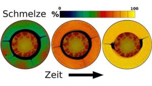
Development of a magma ocean through induction heating in the mantle of exoplanet Trappist-1c. Credit: IWF/ÖAW
Induction heating can completely change the energy budget of an exoplanet and even melt its interior. In a study published by Nature Astronomy an international team led by the Space Research Institute of the Austrian Academy of Sciences with participation of the University of Vienna explains how magma oceans can form under the surface of exoplanets as a result of induction heating.
When a conductive material is embedded in a changing magnetic field, an electrical current is produced inside the body by a process called electromagnetic induction. If the electrical current is strong enough, it can heat the material in which it flows because of electrical resistance. This process called induction heating is widely used in industry to melt materials and at home to cook using induction stoves.
Fast rotation causes heating
An international team led by the Space Research Institute (IWF) of the Austrian Academy of Sciences (OeAW) with participation of the Department of Astrophysics of the University of Vienna was inspired by these examples. “We wanted to investigate if induction heating can play a role on a much bigger scale,” explains first author Kristina Kislyakova. “We were particularly interested in planets orbiting stars that have strong magnetic fields.” These stars can rotate very rapidly, which causes the magnetic field at the planet’s orbit to change rapidly as well. In such cases, induction heating can take place inside the planet.
Impacts on planetary habitability
The team studied low mass stars that exhibit some exotic characteristics in comparison to our Sun. They are much smaller and dimmer. Some of them rotate very fast and possess magnetic fields hundreds of times stronger than the solar one. A good example of such a low-mass star is Trappist-1, which hosts a big family of seven close-in rocky planets, three of which may have liquid water on their surface. This planetary system is a top candidate for the search of Earth-like planets.
Kislyakova and her team have calculated the energy release inside the Trappist-1 planets due to induction heating. “We have shown that for some of the planets, the heating is strong enough to drive enormous volcanic activity or even lead to the formation of a magma ocean beneath the planetary surface.”
As we know from Earth, strong volcanic activity can have a severe influence on a planet’s atmosphere. “Therefore, induction heating can strongly influence the habitability of an exoplanet,” adds IWF co-author Luca Fossati. This new study shows that this effect has to be taken into account when studying the habitability and evolution of planets orbiting low-mass stars.
Reference:
K. G. Kislyakova et al. Magma oceans and enhanced volcanism on TRAPPIST-1 planets due to induction heating, Nature Astronomy (2017). DOI: 10.1038/s41550-017-0284-0
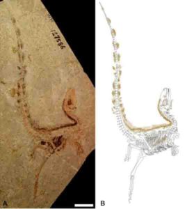
The best-preserved fossil specimen of Sinosauropteryx from the Early Cretaceous Jehol Biota of China and an interpretive drawing of the bones, stomach contents and darkly pigmented feathers. Scale bar represents 50 mm. Credit: University of Bristol
Researchers from the University of Bristol have revealed how a small feathered dinosaur used its colour patterning, including a bandit mask-like stripe across its eyes, to avoid being detected by its predators and prey.
By reconstructing the likely colour patterning of the Chinese dinosaur Sinosauropteryx, researchers have shown that it had multiple types of camouflage which likely helped it to avoid being eaten in a world full of larger meat-eating dinosaurs, including relatives of the infamous Tyrannosaurus Rex, as well as potentially allowing it to sneak up more easily on its own prey.
Fiann Smithwick from the University’s School of Earth Sciences led the work, which has been published today in the journal Current Biology. He said: “Far from all being the lumbering prehistoric grey beasts of past children’s books, at least some dinosaurs showed sophisticated colour patterns to hide from and confuse predators, just like today’s animals.
“Vision was likely very important in dinosaurs, just like today’s birds, and so it is not surprising that they evolved elaborate colour patterns.” The colour patterns also allowed the team to identify the likely habitat in which the dinosaur lived 130 million years ago.
The work involved mapping out how dark pigmented feathers were distributed across the body and revealed some distinctive colour patterns.
These colour patterns can also be seen in modern animals where they serve as different types of camouflage.
The patterns include a dark stripe around the eye, or ‘bandit mask’, which in modern birds helps to hide the eye from would-be predators, and a striped tail that may have been used to confuse both predators and prey.
Senior author, Dr Jakob Vinther, added: “Dinosaurs might be weird in our eyes, but their colour patterns very much resemble modern counterparts.
“They had excellent vision, were fierce predators and would have evolved camouflage patterns like we see in living mammals and birds.”
The small dinosaur also showed a ‘counter-shaded’ pattern with a dark back and light belly; a pattern used by many modern animals to make the body look flatter and less 3D.
This stops animals standing out from their background, making them harder to spot, avoiding detection from would-be predators and potential prey.
Previous work on modern animals, carried out by one of the authors, Bristol’s Professor Innes Cuthill, has shown that the precise pattern of countershading relates to the specific environments in which animals live.
Animals living in open habitats, such as savannahs, often have a counter-shaded pattern that goes from dark to light sharply and high on the side of the body, while those living in more closed habitats, like forests, usually change from dark to light much lower and more gradually.
This principal was applied to Sinosauropteryx, and allowed for the reconstruction of its habitat 130 million years ago. The countershading on Sinosauropteryx went from dark to light high on the body, suggesting that it would be more likely to live in open habitats with minimal vegetation.
Behavioural ecologist Professor Cuthill, who was also a co-author of this study, said: “We’ve shown before that countershading can act as effective camouflage against living predators. It’s exciting that we can now use the colours of extinct animals to predict the sort of environment they lived in.”
Fiann Smithwick added: “By reconstructing the colour of these long-extinct dinosaurs, we have gained a better understanding of not only how they behaved and possible predator-prey dynamics, but also the environments in which they lived.
“This highlights how palaeocolour reconstructions can tell us things not possible from looking at just the bones of these animals.”
Reference:
Fiann M. Smithwick, Robert Nicholls, Innes C. Cuthill, Jakob Vinther. Countershading and Stripes in the Theropod Dinosaur Sinosauropteryx Reveal Heterogeneous Habitats in the Early Cretaceous Jehol Biota. Current Biology, 2017; DOI: 10.1016/j.cub.2017.09.032
Strata of the Chinle Formation below the prominent silcrete horizon exposed in the Petrified Forest National Park. Photo courtesy of Andrew V. Kearns, 2012.
The Norian Chinle Formation in the Southwestern United States provides a snapshot into an ancient terrestrial ecosystem with its famous petrified tree trunks and various plant and vertebrate remains. The fossil plant assemblages, including spores and pollen grains, provide useful information on past vegetation and the response of the vegetation to climate changes.
New pollen and spore data from the Chinle Formation at the Petrified Forest National Park, Arizona, suggest that a extinction of plants occurred between 213 and 217 million years ago in tandem with an extinction of several reptile groups.
The predominance of plants adapted to drier conditions after the extinction event is consistent with the gradual aridification of the North American continent due to the uplift of the Cordilleran volcanic mountain range and the probable northward shift of North America through plate tectonics. Plant community analysis reveals that the floral turnover was followed by the colonization of new plant groups such as the varieties of conifer trees and the decrease in the contribution of seed ferns in the vegetation along waterways.
In their study published in The Geological Society of America Bulletin, Viktoria Baranyi and colleagues propose that the floral reorganization of the riparian communities can be attributed to the gradual climate change and changes in river styles, possibly linked to changes in the mountain chain distributions.
Marked increases in the pollen species e.g., Klausipollenites gouldii, Patinasporites spp. and Froelichsporites traversei are probable indicators of further environmental stress, such as changes of atmospheric pCO2, acid rain, and atmospheric aerosol accumulation due to volcanism in connection with the Pangean rifting and uplift of the Cordilleran mountain chain.
Comparison of the vegetation turnover with younger assemblages from the Chinle Formation in New Mexico reveals similar floral turnover patterns, suggesting their regional significance.
The floral turnover may have affected terrestrial vertebrate communities as the loss of wetland habitat space and an increase in arid climate adapted plants may have dwindled the supply of palatable vegetation for herbivores. The Manicouagan impact event might have contributed to the vegetation change at the Petrified Forest National Park in Arizona but the existing data are unable to prove a direct cause.
Reference:
Viktória Baranyi, Tammo Reichgelt, Paul E. Olsen, William G. Parker, Wolfram M. Kürschner. Norian vegetation history and related environmental changes: New data from the Chinle Formation, Petrified Forest National Park (Arizona, SW USA). GSA Bulletin, 2017; DOI: 10.1130/B31673.1
An illustration of an asteroid impacting Earth. Credit: Image courtesy NASA
Humans have so profoundly altered Earth that, some scientists argue, our current geologic epoch requires a new name: the Anthropocene. But defining the precise start of the era is tricky. Would it begin with the spread of domesticated farm animals or the appearance of radioactive elements from nuclear bomb tests? Scientists report in ACS’ Environmental Science & Technology a method to measure levels of human-made contaminants in sediments that could help pinpoint the Anthropocene’s onset.
The geologic record can sometimes provide clear-cut evidence of epoch changes. For example, when a meteorite collided with Earth 66 million years ago, levels of the metal iridium from the space rock spiked in sediments around the world. This clearly marked the end of the Cretaceous period. However, trying to define the start of the proposed — and much debated — Anthropocene could be more complicated. Human influence over the climate and environment began with the Industrial Revolution in the 1800s, and accelerated dramatically in the second half of the 20th century.
Many markers of human impact on the planet from agriculture, waste disposal and other activities have been archived in the planet’s sedimentary records. The rise in industrial chemicals, such as pesticides and pharmaceuticals, is another example of a human-driven activity that has been captured in sediment layers. To explore the record of synthetic compounds as a possible marker to help define the Anthropocene, Aurea C. Chiaia-Hernández, Juliane Hollender and colleagues turned to a new analytical technique combined with sophisticated data analysis to characterize patterns of contamination over time.
The researchers applied high-resolution mass spectrometry to investigate synthetic chemical contamination in two lakes in Central Europe. They examined 1-meter long cores from each lake bottom, capturing the past 100 years of sediment layers. According to the analysis, the lakes’ sediments contained few synthetic contaminants before the 1950s. But during the 1950s, concentrations of industrial chemicals started to appear in the samples, which is consistent with the boom in industrial activities post-World War II. The researchers say this record clearly demonstrates the beginning of large-scale human impact on the environment. It also shows a decline in contamination following the installation of wastewater treatment plants in the 1970s, providing evidence for successful mitigation measures. Additionally, the introduction of new pollutants that are now finding their way into surface waters can be discovered.
Reference:
Aurea C. Chiaia-Hernández, Barbara F. Günthardt, Martin P. Frey, Juliane Hollender. Unravelling Contaminants in the Anthropocene Using Statistical Analysis of Liquid Chromatography–High-Resolution Mass Spectrometry Nontarget Screening Data Recorded in Lake Sediments. Environmental Science & Technology, 2017; DOI: 10.1021/acs.est.7b03357