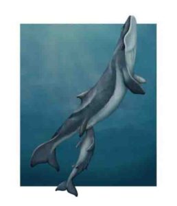
An ancient, dolphin-like marine reptile resembles its distant relative in more than appearance, according to an international team of researchers that includes scientists from North Carolina State University and Sweden’s Lund University. Molecular and microstructural analysis of a Stenopterygius ichthyosaur from the Jurassic (180 million years ago) reveals that these animals were most likely warm-blooded, had insulating blubber and used their coloration as camouflage from predators.
“Ichthyosaurs are interesting because they have many traits in common with dolphins, but are not at all closely related to those sea-dwelling mammals,” says research co-author Mary Schweitzer, professor of biological sciences at NC State with a joint appointment at the North Carolina Museum of Natural Sciences and visiting professor at Lund University. “We aren’t exactly sure of their biology either. They have many features in common with living marine reptiles like sea turtles, but we know from the fossil record that they gave live birth, which is associated with warm-bloodedness. This study reveals some of those biological mysteries.”
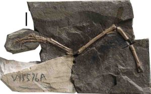
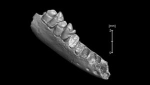
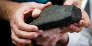
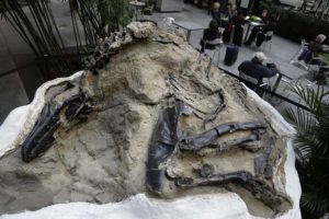
Johan Lindgren, associate professor at Sweden’s Lund University and lead author of a paper describing the work, put together an international team to analyze an approximately 180 million-year-old Stenopterygius fossil from the Holzmaden quarry in Germany.
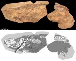
“Both the body outline and remnants of internal organs are clearly visible,” says Lindgren. “Remarkably, the fossil is so well-preserved that it is possible to observe individual cellular layers within its skin.”
Researchers identified cell-like microstructures that held pigment organelles within the fossil’s skin, as well as traces of an internal organ thought to be the liver. They also observed material chemically consistent with vertebrate blubber, which is only found in animals capable of maintaining body temperatures independent of ambient conditions.
Lindgren sent samples from the fossil to international colleagues, including Schweitzer. The team conducted a variety of high-resolution analytical techniques, including time-of-flight secondary ion mass spectrometry (ToF SIMS), nanoscale secondary ion mass spectrometry (NanoSIMS), pyrolysis-gas chromatography/mass spectrometry, as well as immunohistological analysis and various microscopic techniques.
Schweitzer and NC State research assistant Wenxia Zheng extracted soft tissues from the samples and performed multiple, high-resolution immunohistochemical analyses. “We developed a panel of antibodies that we applied to all of the samples, and saw differential binding, meaning the antibodies for a particular protein — like keratin or hemoglobin — only bound to particular areas,” Schweitzer says. “This demonstrates the specificity of these antibodies and is strong evidence that different proteins persist in different tissues. You wouldn’t expect to find keratin in the liver, for example, but you would expect hemoglobin. And that’s what we saw in the responses of these samples to different antibodies and other chemical tools.”
Lindgren’s lab also found chemical evidence for subcutaneous blubber. “This is the first direct, chemical evidence for warm-bloodedness in an ichthyosaur, because blubber is a feature of warm-blooded animals,” Schweitzer says.
Taken together, the researchers’ findings indicate that the Stenopterygius had skin similar to that of a whale, and coloration similar to many living marine animals — dark on top and lighter on the bottom — which would provide camouflage from predators, like pterosaurs from above, or pliosaurs from below.
“Both morphologically and chemically, we found that although Stenopterygius would be loosely considered ‘reptiles,’ they lost the scaly skin associated with these animals — just as the modern leatherback sea turtle has,” Schweitzer says. “Losing the scales reduces drag and increases maneuverability underwater.
“This animal’s preservation is unusual, especially for a marine environment — but then, the Holzmaden formation is known for its exceptional preservation. This specimen has given us more evidence that these tissues and molecules can preserve for extremely long periods, and that soft tissue analysis can shed light on evolutionary patterns, relationships, and how ancient animals functioned in their environment.
“Our results were repeatable and consistent across labs. This work really shows what we’re capable of discovering when we perform a multidisciplinary, multi-institutional study of an exceptional specimen.”
Reference:
Johan Lindgren, Peter Sjövall, Volker Thiel, Wenxia Zheng, Shosuke Ito, Kazumasa Wakamatsu, Rolf Hauff, Benjamin P. Kear, Anders Engdahl, Carl Alwmark, Mats E. Eriksson, Martin Jarenmark, Sven Sachs, Per E. Ahlberg, Federica Marone, Takeo Kuriyama, Ola Gustafsson, Per Malmberg, Aurélien Thomen, Irene Rodríguez-Meizoso, Per Uvdal, Makoto Ojika, Mary H. Schweitzer. Soft-tissue evidence for homeothermy and crypsis in a Jurassic ichthyosaur. Nature, 2018; DOI: 10.1038/s41586-018-0775-x
Note: The above post is reprinted from materials provided by North Carolina State University.