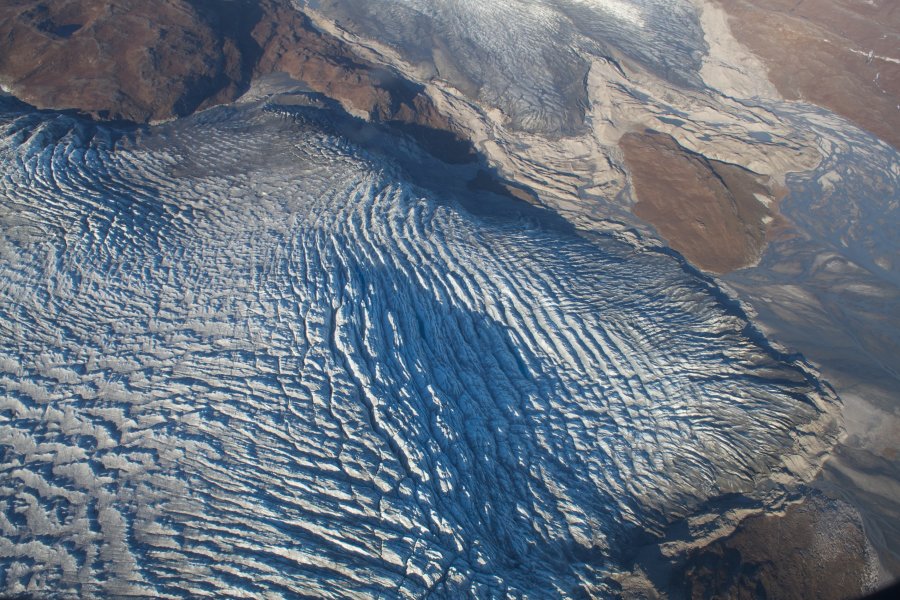
Crevassed glacier terminus in West Greenland. Credit: Sam Doyle
According to a new study published in Nature Geoscience, the Greenland ice sheet has been shown to accelerate in response to surface rainfall and melt associated with late-summer and autumnal cyclonic weather events.
Samuel Doyle and an international team of colleagues led from Aberystwyth University’s Centre for Glaciology combined records of ice motion, water pressure at the ice sheet bed, and river discharge with surface meteorology across the western margin of the Greenland ice sheet and captured the wide-scale effects of an unusual week of warm, wet weather in late August and early September, 2011.
They found that the cyclonic weather system led to extreme surface runoff — a combination of ice melt and rain — that overwhelmed the ice sheet’s basal drainage system, driving a marked increase in ice flow across the entire western sector of the ice sheet and extending 140 km into the ice sheet’s interior.
“It is like an urban sewerage system that is temporarily overwhelmed by an intense rain-storm. The ice sheet plumbing — literally a network of pipes, cavities and channels — gets backed up by the sheer quantity of runoff draining into it, leading to flooding and high water pressures, which literally hydraulically lifts the ice sheet up off its bed, reducing basal friction and sending it on its way,” said Prof Alun Hubbard the principal investigator who led the 4-year project which was funded by Natural Environment Research Council (NERC) and the Royal Geographical Society amongst others.
This particular depression prevailed across a broad swathe of southern and western Greenland, and a correspondingly-widespread acceleration in ice motion was reported from all available satellite and GPS tracking stations. This response was apparent at glaciers that terminate on dry land as well as those that calve into the sea.
Cyclonic systems, or depressions, are no great surprise to us in the UK and western Europe where, even in summer, they are unfortunately part and parcel of our everyday weather — commonly bringing wind and rain. In contrast, such conditions are less common across Greenland, which is normally dominated by a stable, high-pressure system centred over the ice sheet.
The influence of such rainfall events has not, until now, been considered in assessments of the melt and flow response of any ice sheet. This is an important omission because, although such cyclonic conditions are currently rare across Greenland, they are predicted to increase in the future, therefore likely playing an increasing role in driving mass loss from the Greenland ice sheet, which currently contributes over 0.7 mm per year to global sea-level — a rate at least double that of Antarctica.
“The late-summer timing was critical. The event occurred after the end of the melt season and the ice-sheet’s drainage system had started to close down. In this state the ice sheet’s drainage system just couldn’t cope,” said Dr Samuel Doyle, lead author of the study.
Since the 1980s when rainfall measurements began in the west Greenland town of Kangerlussuaq, the focus of the study, the proportion of precipitation now falling as rain rather than snow has both increased and extended into the late summer and autumn in line with increased circulation and moisture availability within a warmer, more energetic atmosphere.
“We’re seeing that warm wet weather is increasing with climate change and is driving more melt of the Greenland ice-sheet than we thought. And worryingly, this melt is now reaching ever higher elevations on the ice sheet” says Prof. Jason Box, one of the co- authors of the study.
“The jury is out as to whether the ‘rainfall’ events identified in our study had a lasting influence on the evolution of the Greenland ice sheet. Just like in many regions of the planet, observed climate warming doesn’t just mean hotter summers and milder winters; it’s more complex than that and more often it means more intense storm events at unusual times of the year just like we’ve witnessed here in the UK. These events are predicted to increase in the future and under a succession of such autumnal storm events there is no doubt the ice sheet will experience accelerated melt and flow which could only hasten its eventual demise,” commented Alun Hubbard.
Reference:
Samuel H. Doyle, Alun Hubbard, Roderik S.W. van de Wal, Jason E. Box, Dirk van As, Killian Scharrer, Toby W. Meierbachtol, Paul C.J.P. Smeets, Joel T. Harper, Emma Johansson, Ruth H. Mottram, Andreas B. Mikkelsen, Frank Wilhelms, Henry Patton, Poul Christoffersen, and Bryn Hubbard. Amplified melt and flow of the Greenland ice sheet driven by late-summer cyclonic rainfall. Nature Geoscience, July 2015 DOI: 10.1038/ngeo2482
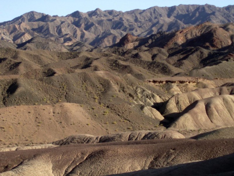
July GSA Today cover image: Khosoumi Mountains in the southern part of the Chapedony metamorphic core complex of Central Iran. The high mountains in the back are represented by Eocene plutonic rocks of the footwall unit. Eocene volcaniclastic rocks in the foreground form the hanging-wall unit. Credit: Franz Neubauer of the University of Salzburg and Fariba Kargaranbafghi of the University of Yazd, and GSA Today.
In the July issue of GSA Today, Franz Neubauer of the University of Salzburg and Fariba Kargaranbafghi of the University of Yazd describe thinning of the lithosphere that they associate with the formation of a metamorphic core complex in the Central Iranian plateau.
The core complex is located within a continental rift and was exhumed at a rate of approx. 0.75 to 1.3 km per million years during the main phase of oceanic subduction of the Arabian plate beneath the Central Iranian block between ca. 30 and 49 million years ago.
The authors indicate that lithosphere and continental crust were thinned beneath regions of surface extension.
The thinning of the underlying lithosphere appears to have been compensated by hot asthenosphere, as indicated by low seismic velocities in the Central Iranian block.
The authors conclude that the development of the core complex involved lithospheric removal associated with extension and upwelling of hot asthenosphere. Later processes, like slab break-off and associated uplift of the Central Iranian plateau, may have modified the structure.
Reference:
Fariba Kargaranbafghi, Franz Neubauer. Lithospheric thinning associated with formation of a metamorphic core complex and subsequent formation of the Iranian plateau. GSA Today, 2015; 4 DOI: 10.1130/GSATG229A.1
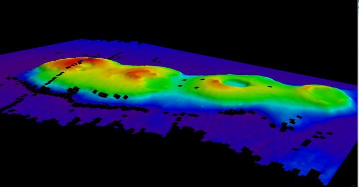
Australia’s new ocean-going research vessel Investigator has discovered extinct volcanoes likely to be 50 million years old about 250 kilometres off the coast of Sydney. The largest is 1.5 kilometres across the rim and rises 700 metres from the sea floor. Credit: Marine National Facility
Australia’s new ocean-going research vessel Investigator has discovered extinct volcanoes likely to be 50 million years old about 250 kilometres off the coast of Sydney.
The chief scientist for the voyage, UNSW Australia marine biologist Professor Iain Suthers, said the volcanoes were discovered in 4,900 meters of water during a search for nursery grounds for larval lobsters. At the same time the ship was also routinely mapping the seafloor.
“The voyage was enormously successful. Not only did we discover a cluster of volcanoes on Sydney’s doorstep, we were amazed to find that an eddy off Sydney was a hotspot for lobster larvae at a time of the year when we were not expecting them,” Professor Suthers said.
The four extinct volcanoes in the cluster are calderas, which form after a volcano erupts and the land around them collapses, forming a crater. The largest is 1.5 kilometres across the rim and it rises 700 metres from the sea floor.
Professor Richard Arculus from the Australian National University, an igneous petrologist and a world-leading expert on volcanoes, said these particular types of volcanoes are really important to geoscientists because they are like windows into the seafloor.
“They tell us part of the story of how New Zealand and Australia separated around 40-80 million years ago and they’ll now help scientists target future exploration of the sea floor to unlock the secrets of the Earth’s crust,” Professor Arculus said.
“They haven’t been found before now because the sonar on the previous Marine National Facility (MNF) research vessel, Southern Surveyor, could only map the sea floor to 3,000 metres, which left half of Australia’s ocean territory out of reach.” ”
On board the new MNF vessel, Investigator, we have sonar that can map the sea floor to any depth, so all of Australia’s vast ocean territory is now within reach, and that is enormously exciting,” Professor Arculus said.
Professor Suthers said the 94-metre Investigator has other capabilities that marine scientists in Australia have never had before, and the vessel will be key to unlocking the secrets of the oceans around our continent and beyond.
“Investigator is able to send and receive data while we’re at sea, which meant the team back on base at UNSW in Sydney could analyse the information we were collecting at sea and send back their analysis, along with satellite imagery, so we could chase the eddies as they formed,” Professor Suthers said.
“This is the first time we’ve been able to respond directly to the changing dynamics of the ocean and, for a biological oceanographer like me, it doesn’t get more thrilling,” Professor Suthers said.
“It was astounding to find juvenile commercial fish species like bream and tailor 150 kilometres offshore, as we had thought that once they were swept out to sea that was end of them. But in fact these eddies are nursery grounds along the east coast of Australia.”
The research voyage led by Professor Iain Suthers departed Brisbane on 3 June and concluded on 18 June in Sydney, with 28 scientists from UNSW, La Trobe University, the University of British Columbia, the University of Sydney, the University of Auckland, the University of Technology Sydney, and Southern Cross University.
The centre of the volcanic cluster is 33 31 S, 153 52 E, which is 248 kilometres from Sydney Heads. The cluster is 20 kilometres long and six kilometres wide and the seafloor is 4890 metres deep, with the highest point in the cluster rising up to 3,998 metres.
Video
UNSW Researchers discovered a volcanic cluster off the coast of Sydney in 2015 at 33 31 S, 153 52 E.
The RV Investigator crew have discovered extinct volcanoes likely to be 50 million years old, about 250 km off the coast of Sydney in 4,900 m of water. While scientists were searching for the nursery grounds for larval lobsters, the ship was also routinely mapping the seafloor when the volcanoes were discovered. They haven’t been found before now, because the sonar on the previous Marine National Facility (MNF) research vessel, Southern Surveyor, could only map the sea floor to 3,000 m, which left half of Australia’s ocean territory out of reach. The centre of the volcanic cluster is 33 31 S, 153 52 E, which is 248 km from Sydney Heads. The cluster is 20 km long and six km wide and the seafloor 4890 metres deep, with the highest point in the cluster rising up to 3998 metres.
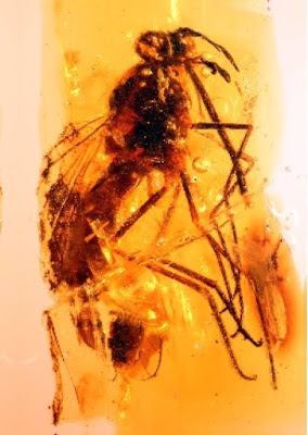
A piece of amber from El Soplao cave with a specimen of the species Buccinatormyia magnifica. Credit: Image courtesy of Universidad de Barcelona
When we think about pollination, the image that comes first to our mind is a bee or a butterfly covered by pollen. However, in the Cretaceous — about 105 million years ago — bees and butterflies did not exist, and most terrestrial ecosystems were dominated by non-flowering plants (gymnosperms).
An international research team has recently discovered some amber fly specimens in El Soplao cave (Cantabria, Spain). According to an article published in the scientific journal Current Biology, these specimens fed on nectar and pollinized gymnosperm plants 105 million years ago. Xavier Delclòs, professor in the Department ofStratigraphy, Paleontology and Marine Geosciences and researcher at the Biodiversity Research Institute (IRBio) of the University of Barcelona, is one of the authors of the study. The article is also authored by Enrique Peñalver and Eduardo Barron (Geological and Mining Institute of Spain, IGME); Antonio Arillo (Complutense University of Madrid, UCM); David Grimaldi (American Museum of Natural History); Ricardo Pérez de la Fuente (Harvard University, USA,) and Mark L. Riccioi (Cornell (University, USA).
Plants and insects: a long history
Plants attract insects with different strategies — for example, with their sweet and nutritious nectar — in order to get them transport pollen and enable the process of pollination. By this way, plants and insects establish a fundamental symbiotic relationship that plays a key role in the preservation of terrestrial ecosystems. Besides bees and other similar species, the most important pollinators in current ecosystems — where flowering plants predominate — are proboscid butterflies, beetles, thrips and flies. On the contrary, in Cretaceous landscapes, dominant species were gymnosperms (for examples, pines, firs, cycads) and the main agent of pollination was the wind.
Flies that pollinated Cretaceous plants
Amber from El Soplao (Cantabria) is providing traces of new insect species key to understand how was life in Cretaceous forests, when today’s Iberian Peninsula was a giant island. The study describes two species of flies, well preserved in amber, which present a long specialized proboscis and belong to the family Zhangsolvidae, extinct before dinosaurs. One of the specimens has hundreds of grains from a Bennettitalean species, an extinct order of gymnosperms.
The study proves that the internal structure of flies’ proboscis has been preserved at a microscopic level, according to evidence provided by computed tomography and transmission electron microscopy. The scientific team has showed that these flies took nectar from plants by approaching them in beating flight, like hummingbirds do.
When angiosperms began to dominate terrestrial ecosystems
There are few known cases of insects that fossilized when they were transporting pollen from one flower to another. The new fossils found in Cantabria show that flies and Bennettitales held a close partnership 105 million years ago. Why amber insects carrying angiosperm pollen have not been found? According to experts, this is an outstanding scientific finding because at that moment angiosperms were beginning to dominate terrestrial ecosystems and diversify in many species.
“If insects were able to feed on gymnosperms flower structures, it is probably true that the transition to angiosperms took place then,” affirm the authors of the study.
Video
Reference:
Enrique Peñalver, Antonio Arillo, Ricardo Pérez-de la Fuente, Mark L. Riccio, Xavier Delclòs, Eduardo Barrón, David A. Grimaldi. Long-Proboscid Flies as Pollinators of Cretaceous Gymnosperms. Current Biology, 2015; DOI: 10.1016/j.cub.2015.05.062
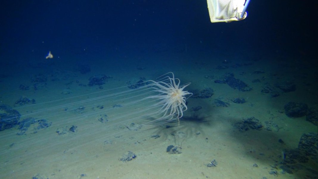
Relicanthus sp. — a new species from a new order of Cnidaria collected at 4,100 meters in the Clarion-Clipperton Fracture Zone (CCZ) that lives on sponge stalks attached to nodules. Credit: Craig Smith and Diva Amon, ABYSSLINE Project
Thousands of feet below the ocean’s surface lies a hidden world of undiscovered species and unique seabed habitats–as well as a vast untapped store of natural resources including valuable metals and rare-earth minerals. Technology and infrastructure development worldwide is dramatically increasing demand for these resources, which are key components in everything from cars and modern buildings to computers and smartphones. This demand has catalyzed interest in mining huge areas of the deep-sea floor.
In a paper published this week in Science, researchers from the Center for Ocean Solutions and co-authors from leading institutions around the world propose a strategy for balancing commercial extraction of deep-sea resources with protection of diverse seabed habitats. The paper is intended to inform upcoming discussions by the International Seabed Authority (ISA) that will set the groundwork for future deep-sea environmental protection and mining regulations.
“Our purpose is to point out that the ISA has an important opportunity to create networks of no-mining Marine Protected Areas (MPAs) as part of the regulatory framework they are considering at their July meeting,” says lead author Lisa Wedding, an early career science fellow at the Center for Ocean Solutions. “The establishment of regional MPA networks in the deep sea could potentially benefit both mining and biodiversity interests by providing more economic certainty and ecosystem protection.”
The ISA is charged with managing the seabed and its resources outside of national jurisdictions for the benefit of humankind. According to the United Nations Convention on the Law of the Sea (UNCLOS), the deep seabed is legally a part of the “common heritage of humankind,” meaning that it belongs to each and every human on the planet.
“The ISA is the only body with the legal standing and responsibility to manage mining beyond national jurisdiction,” said Kristina Gjerde, an international high-seas lawyer and co-author on the Science paper.
Since 2001, the ISA has granted 26 mining exploration contracts covering more than one million square kilometers of seabed, with 18 of these contracts granted in the last four years. Researchers recommend that the ISA, as part of its strategic plans to protect deep-seabed habitats and manage mining impacts, take a precautionary approach and set up networks of MPAs before additional large claim areas are granted for deep seabed mining.
“Given our paltry understanding of deep-sea environments, regional networks of MPAs that designate significant portions of the deep seabed as off-limits to mining would provide key insurance against unanticipated environmental impacts,” said co-author Steven Gaines, dean of the Bren School of Environmental Science & Management at the University of California at Santa Barbara.
Mining impacts could affect important environmental benefits that the deep sea provides to human beings. For example, the deep sea is a key player in our planet’s carbon cycle, capturing a substantial amount of human-emitted carbon which impacts both weather and climate. Mining activities could disturb these deep-sea carbon sinks, releasing excess carbon back into the atmosphere. The deep sea also sustains economically important fisheries, and harbors microorganisms which have proven valuable in a number of pharmaceutical, medical and industrial applications.
“Deep-sea areas targeted by mining claims frequently harbor high biodiversity and fragile habitats, and may have very slow rates of recovery from physical disturbance,” said Craig Smith, a co-author and professor of oceanography at the University of Hawaii at Manoa. Smith and a team of scientists, helped the ISA pioneer the deep sea’s first regional environmental management plan in 2012. Located in an area of the Pacific Ocean known as the Clarion-Clipperton Zone (CCZ), the plan honored existing mining exploration claims while protecting delicate habitats by creating a network of MPAs. The CCZ serves as a model for how future deep-sea ecosystem management could unfold.
“This kind of precautionary approach achieves a balance of economic interests and conservation benefits,” said Sarah Reiter, a co-author and former early career law and policy fellow at the Center for Ocean Solutions who now works as an ocean policy analyst at the Monterey Bay Aquarium.
The upcoming ISA session on July 15th represents a critical juncture for defining the future of deep-sea mining and protection.
“The time is now to protect this important part of the planet for current and future generations,” said Larry Crowder, a co-author and science director at the Center for Ocean Solutions and senior fellow at the Stanford Woods Institute for the Environment. “Decisions that affect us all will be made by the ISA this summer.”
Reference:
L. M. Wedding, S. M. Reiter, C. R. Smith, K. M. Gjerde, J. N. Kittinger, A. M. Friedlander, S. D. Gaines, M. R. Clark, A. M. Thurnherr, S. M. Hardy, and L. B. Crowder. Managing mining of the deep seabed. Science, July 2015 DOI: 10.1126/science.aac6647
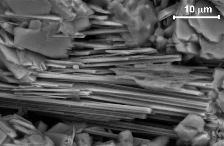
The presence of the mineral actinolite in the caprock of Campi Flegrei provided the crucial clue to unraveling the chemical processes that formed the concrete-like rock beneath the caldera. Credit: Courtesy of Tiziana Vanorio
The discovery of a fiber-reinforced, concrete-like rock formed in the depths of a dormant supervolcano could help explain the unusual ground swelling that led to the evacuation of an Italian port city and inspire durable building materials in the future, Stanford scientists say.
The “natural concrete” at the Campi Flegrei volcano is similar to Roman concrete, a legendary compound invented by the Romans and used to construct the Pantheon, the Coliseum, and ancient shipping ports throughout the Mediterranean.
“This implies the existence of a natural process in the subsurface of Campi Flegrei that is similar to the one that is used to produce concrete,” said Tiziana Vanorio, an experimental geophysicist at Stanford’s School of Earth, Energy & Environmental Sciences.
Campi Flegrei lies at the center of a large depression, or caldera, that is pockmarked by craters formed during past eruptions, the last of which occurred nearly 500 years ago. Nestled within this caldera is the colorful port city of Pozzuoli, which was founded in 600 B.C. by the Greeks and called “Puteoli” by the Romans.
Beginning in 1982, the ground beneath Pozzuoli began rising at an alarming rate. Within a two-year span, the uplift exceeded six feet-an amount unprecedented anywhere in the world. “The rising sea bottom rendered the Bay of Pozzuoli too shallow for large craft,” Vanorio said.
Making matters worse, the ground swelling was accompanied by swarms of micro-earthquakes. Many of the tremors were too small to be felt, but when a magnitude 4 quake juddered Pozzuoli, officials evacuated the city’s historic downtown. Pozzuoli became a ghost town overnight.
A teenager at the time, Vanorio was among the approximately 40,000 residents forced to flee Pozzuoli and settle in towns scattered between Naples and Rome. The event made an impression on the young Vanorio, and inspired her interests in the geosciences. Now an assistant professor at Stanford, Vanorio decided to apply her knowledge about how rocks in the deep Earth respond to mechanical and chemical changes to investigate how the ground beneath Pozzuoli was able to withstand so much warping before cracking and setting off micro-earthquakes.
“Ground swelling occurs at other calderas such as Yellowstone or Long Valley in the United States, but never to this degree, and it usually requires far less uplift to trigger earthquakes at other places,” Vanorio said. “At Campi Flegrei, the micro-earthquakes were delayed by months despite really large ground deformations.”
To understand why the surface of the caldera was able to accommodate incredible strain without suddenly cracking, Vanorio and a post-doctoral associate, Waruntorn Kanitpanyacharoen, studied rock cores from the region. In the early 1980s, a deep drilling program probed the active geothermal system of Campi Flegrei to a depth of about 2 miles. When the pair analyzed the rock samples, they discovered that Campi Flegrei’s caprock-a hard rock layer located near the caldera’s surface-is rich in pozzolana, or volcanic ash from the region.
The scientists also noticed that the caprock contained tobermorite and ettringite-fibrous minerals that are also found in manmade concrete. These minerals would have made Campi Flegrei’s caprock more ductile, and their presence explains why the ground beneath Pozzuoli was able to withstand significant bending before breaking and shearing. But how did tobermorite and ettringite come to form in the caprock?
Once again, the drill cores provided the crucial clue. The samples showed that the deep basement of the caldera-the “wall” of the bowl-like depression-consisted of carbonate-bearing rocks similar to limestone, and that interspersed within the carbonate rocks was a needle-shaped mineral called actinolite.
“The actinolite was the key to understanding all of the other chemical reactions that had to take place to form the natural cement at Campi Flegrei,” said Kanitpanyacharoen, who is now at Chulalongkorn University in Thailand.
From the actinolite and graphite, the scientists deduced that a chemical reaction called decarbonation was occurring beneath Campi Flegrei. They believe that the combination of heat and circulating mineral-rich waters decarbonates the deep basement, prompting the formation of actinolite as well as carbon dioxide gas. As the CO2 mixes with calcium-carbonate and hydrogen in the basement rocks, it triggers a chemical cascade that produces several compounds, one of which is calcium hydroxide. Calcium hydroxide, also known as portlandite or hydrated lime, is one of the two key ingredients in manmade concrete, including Roman concrete. Circulating geothermal fluids transport this naturally occurring lime up to shallower depths, where it combines with the pozzolana ash in the caprock to form an impenetrable, concrete-like rock capable of withstanding very strong forces.
“This is the same chemical reaction that the ancient Romans unwittingly exploited to create their famous concrete, but in Campi Flegrei it happens naturally,” Vanorio said.
In fact, Vanorio suspects that the inspiration for Roman concrete came from observing interactions between the volcanic ash at Pozzuoli and seawater in the region. The Roman philosopher Seneca, for example, noted that the “dust at Puteoli becomes stone if it touches water.”
“The Romans were keen observers of the natural world and fine empiricists,” Vanorio said. “Seneca, and before him Vitruvius, understood that there was something special about the ash at Pozzuoli, and the Romans used the pozzolana to create their own concrete, albeit with a different source of lime.”
Pozzuoli was the main commercial and military port for the Roman Empire, and it was common for ships to use pozzolana as ballast while trading grain from the eastern Mediterranean. As a result of this practice, volcanic ash from Campi Flegrei-and the use of Roman concrete-spread across the ancient world. Archeologists have recently found that piers in Alexandria, Caesarea, and Cyprus are all made from Roman concrete and have pozzolana as a primary ingredient.
Interestingly, the same chemical reaction that is responsible for the unique properties of the Campi Flegrei’s caprock can also trigger its downfall. If too much decarbonation occurs-as might happen if a large amount of saltwater, or brine, gets injected into the system-an excess of carbon dioxide, methane and steam is produced. As these gases rise toward the surface, they bump up against the natural cement layer, warping the caprock. This is what lifted Pozzuoli in the 1980s. When strain from the pressure buildup exceeded the strength of the caprock, the rock sheared and cracked, setting off swarms of micro-earthquakes. As pent-up gases and fluids vent into the atmosphere, the ground swelling subsided. Vanorio and Kanitpanyacharoen suspect that as more calcium hydroxide was produced at depth and transported to the surface, the damaged caprock was slowly repaired, its cracks “healed” as more natural cement was produced.
Vanorio believes the conditions and processes responsible for the exceptional rock properties at Campi Flegrei could be present at other calderas around the world. A better understanding of the conditions and processes that formed Campi Flegrei’s caprock could also allow scientists to recreate it in the lab, and perhaps even improve upon it to engineer more durable and resilient concretes that are better able to withstand large stresses and shaking, or to heal themselves after damage.
“There is a need for eco-friendly materials and concretes that can accommodate stresses more easily,” Vanorio said. “For example, extracting natural gas by hydraulic fracturing can cause rapid stress changes that cause concrete well casings to fail and lead to gas leaks and water contamination.”
Video
The discovery beneath Campi Flegrei, a dormant supervolcano in southern Italy, of a concrete-like rock that is similar to Roman concrete explains why the ground beneath the town of Pozzuoli rose by several meters in the 1980s, forcing the evacuation of 40,000 people.
A series of chemical reactions occurring beneath Italy’s Campi Flegrei is creating lime that then reacts with volcanic ash in the caprock to form a concrete-like substance.
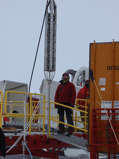
UCSC researchers lowered a geothermal probe through a borehole in the West Antarctic ice sheet to measure temperatures in the sediments beneath half a mile of ice. Credit: WISSARD/UCSC
The amount of heat flowing toward the base of the West Antarctic ice sheet from geothermal sources deep within the Earth is surprisingly high, according to a new study led by UC Santa Cruz researchers. The results, published July 10 in Science Advances, provide important data for researchers trying to predict the fate of the ice sheet, which has experienced rapid melting over the past decade.
Lead author Andrew Fisher, professor of Earth and planetary sciences at UC Santa Cruz, emphasized that the geothermal heating reported in this study does not explain the alarming loss of ice from West Antarctica that has been documented by other researchers. “The ice sheet developed and evolved with the geothermal heat flux coming up from below—it’s part of the system. But this could help explain why the ice sheet is so unstable. When you add the effects of global warming, things can start to change quickly,” he said.
High heat flow below the West Antarctic ice sheet may also help explain the presence of lakes beneath it and why parts of the ice sheet flow rapidly as ice streams. Water at the base of the ice streams is thought to provide the lubrication that speeds their motion, carrying large volumes of ice out onto the floating ice shelves at the edges of the ice sheet. Fisher noted that the geothermal measurement was from only one location, and heat flux is likely to vary from place to place beneath the ice sheet.
“This is the first geothermal heat flux measurement made below the West Antarctic ice sheet, so we don’t know how localized these warm geothermal conditions might be. This is a region where there is volcanic activity, so this measurement may be due to a local heat source in the crust,” Fisher said.
The study was part of a large Antarctic drilling project funded by the National Science Foundation called WISSARD (Whillans Ice Stream Subglacial Access Research Drilling), for which UC Santa Cruz is one of three lead institutions. The research team used a special thermal probe, designed and built at UC Santa Cruz, to measure temperatures in sediments below Subglacial Lake Whillans, which lies beneath half a mile of ice. After boring through the ice sheet with a special hot-water drill, researchers lowered the probe through the borehole until it buried itself in the sediments below the subglacial lake. The probe measured temperatures at different depths in the sediments, revealing a rate of change in temperature with depth about five times higher than that typically found on continents. The results indicate a relatively rapid flow of heat towards the bottom of the ice sheet.
This geothermal heating contributes to melting of basal ice, which supplies water to a network of subglacial lakes and wetlands that scientists have discovered underlies a large region of the ice sheet. In a separate study published last year in Nature, the WISSARD microbiology team reported an abundant and diverse microbial ecosystem in the same lake. Warm geothermal conditions may help to make subglacial habitats more supportive of microbial life, and could also drive fluid flow that delivers heat, carbon, and nutrients to these communities.
According to coauthor Slawek Tulaczyk, professor of Earth and planetary sciences at UC Santa Cruz and one of the WISSARD project leaders, the geothermal heat flux is an important value for the computer models scientists are using to understand why and how quickly the West Antarctic ice sheet is shrinking.
“It is important that we get this number right if we are going to make accurate predictions of how the West Antarctic ice sheet will behave in the future, how much it is melting, how quickly ice streams flow, and what the impact might be on sea level rise,” Tulaczyk said. “I waited for many years to see a directly measured value of geothermal flux from beneath this ice sheet.”
Antarctica’s huge ice sheets are fed by snow falling in the interior of the continent. The ice gradually flows out toward the edges. The West Antarctic ice sheet is considered less stable than the larger East Antarctic ice sheet because much of it rests on land that is below sea level, and the ice shelves at its outer edges are floating on the sea. Recent studies by other research teams have found that the ice shelves are melting due to warm ocean currents now circulating under the ice, and the rate at which the ice shelves are shrinking is accelerating. These findings have heightened concerns about the overall stability of the West Antarctic ice sheet.
The geothermal heat flux measured in the new study was about 285 milliwatts per square meter, which is like the heat from one small LED Christmas-tree light per square meter, Fisher said. The researchers also measured the upward heat flux through the ice sheet (about 105 milliwatts per square meter) using an instrument developed by coauthor Scott Tyler at the University of Nevada, Reno. That instrument was left behind in the WISSARD borehole as it refroze, and the measurements, based on laser light scattering in a fiber-optic cable, were taken a year later. Combining the measurements both below and within the ice enabled calculation of the rate at which melt water is produced at the base of the ice sheet at the drill site, yielding a rate of about half an inch per year.
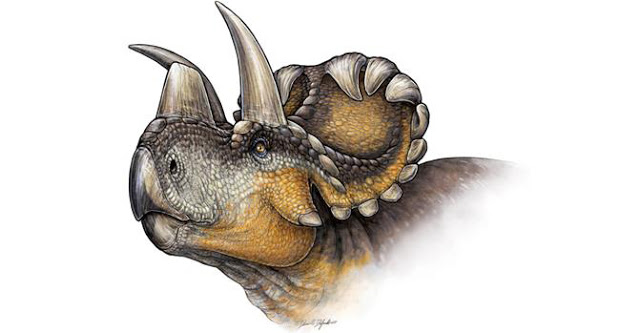
This is a ife reconstruction of Wendiceratops pinhornensis. Credit: Danielle Dufault
Scientists have discovered a striking new species of horned dinosaur (ceratopsian) based on fossils collected from a bone bed in southern Alberta, Canada. Wendiceratops (WEN-dee-SARE-ah-TOPS) pinhornensis was approximately 6 meters (20 feet) long and weighed more than a ton. It lived about 79 million years ago, making it one of the oldest known members of the family of large-bodied horned dinosaurs that includes the famous Triceratops, the Ceratopsidae. Research describing the new species is published online in the open access journal, PLOS ONE.
The new dinosaur, named Wendiceratops pinhornensis, is described from over 200 bones representing the remains of at least four individuals (three adults and one juvenile) collected from a bonebed in the Oldman Formation of southern Alberta, near the border with Montana, USA. It was a herbivore, and would crop low-lying plants with a parrot-like beak, and slice them up with dozens of leaf-shaped teeth. Wendiceratops had a fantastically adorned skull, particularly for an early member of the horned dinosaur family. Its most distinctive feature is a series of forward-curling hook-like horns along the margin of the wide, shield-like frill that projects from the back of its skull. The new find ranks among other recent discoveries in having some of the most spectacular skull ornamentation in the horned dinosaur group.
“Wendiceratops helps us understand the early evolution of skull ornamentation in an iconic group of dinosaurs characterized by their horned faces,” said Dr. David Evans, Temerty Chair and Curator of Vertebrate Palaeontology at the Royal Ontario Museum in Toronto, Canada, and co-author of the study. “The wide frill of Wendiceratops is ringed by numerous curled horns, the nose had a large, upright horn, and it’s likely there were horns over the eyes too. The number of gnarly frill projections and horns makes it one of the most striking horned dinosaurs ever found.”
The horn on the nose is the most interesting feature of Wendiceratops. Although the nasal bone is represented by fragmentary specimens and its complete shape is unknown, it is clear that it supported a prominent, upright nasal horncore. This represents the earliest documented occurrence of a tall nose horn in Ceratopsia. Not only does it tell scientists when the nose horn evolved, the research reveals that an enlarged conical nasal horn evolved at least twice in the horned dinosaur family, once in the short-frilled Centrosaurinae group that includes Wendiceratops, and again in the long-frilled Chasmosaurinae group which includes Triceratops. A nose horn has been generally thought to characterize Ceratopsidae, and be present in their common ancestor.
“Beyond its odd, hook-like frill, Wendiceratops has a unique horn ornamentation above its nose that shows the intermediate evolutionary development between low, rounded forms of the earliest horned dinosaurs and the large, tall horns of Styracosaurus, and its relatives,” said Dr. Michael Ryan, Curator of Vertebrate Paleontology at the Cleveland Museum of Natural History, and co-author of the study. “The locked horns of two Wendiceratops could have been used in combat between males to gain access to territory or females.”
The recognition of Wendiceratops affirms a high diversity of ceratopsids likely associated with a rapid evolutionary radiation in the group. It also helps document high faunal turnover rates of ceratopsid taxa early in their evolution, coupled with some degree of ecological niche partitioning during this time.
The name Wendiceratops (Wendi + ceratops) means “Wendy’s horned-face,” and celebrates renowned Alberta fossil hunter Wendy Sloboda, who discovered the site in 2010. This is a well-deserved honor for Sloboda, who has discovered hundreds of important fossils in the last three decades, including several new species. “Wendy Sloboda has a sixth sense for discovering important fossils. She is easily one of the very best dinosaur hunters in the world,” said Evans.
This dinosaur is the latest in a series of new finds being made by Evans and Ryan as part of their Southern Alberta Dinosaur Project, which is designed to fill in gaps in our knowledge of Late Cretaceous dinosaurs in North America and study their evolution. This project focuses on the paleontology of some of oldest dinosaur-bearing rocks in Alberta, as well as rocks of neighboring Montana that are of the same age. A full-sized skeleton and exhibit profiling Wendiceratops is currently on display at the Royal Ontario Museum in Toronto, and the dig uncovering it appeared in the HISTORY Channel documentary series Dino Hunt Canada.
Video
Reference:
David C. Evans, Michael J. Ryan. Cranial Anatomy of Wendiceratops pinhornensis gen. et sp. nov., a Centrosaurine Ceratopsid (Dinosauria: Ornithischia) from the Oldman Formation (Campanian), Alberta, Canada, and the Evolution of Ceratopsid Nasal Ornamentation. PLOS ONE, 2015; 10 (7): e0130007 DOI: 10.1371/journal.pone.0130007
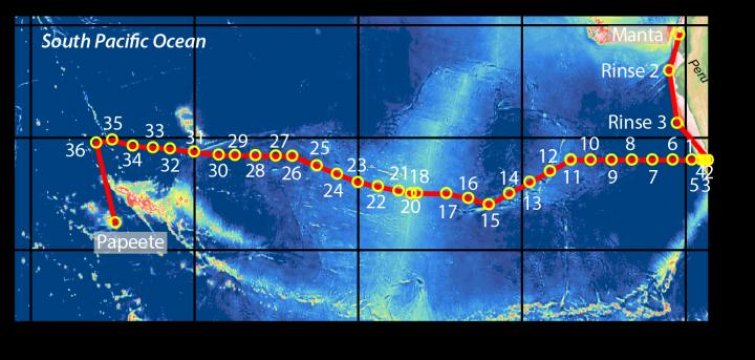
The 57-day voyage in late 2013 followed a route where previous research had followed the track of hydrothermal fluids. Credit: J. Resing / Univ. of Washington
At the bottom of the sea, volcanic and magmatic forces create hot springs that spew super-heated water into the deep sea. The hot, acidic water scours metals from Earth’s crust, and the warm chemical-rich water from these remote geysers supports exotic deep-sea ecosystems.
It had been widely thought the story stopped there. Metals such as iron and manganese were thought to quickly react and form particles that would either clump together or stick to other things, causing them to sink to the seafloor close to the source. But new research proves that the metals remain dissolved and follow deep-sea currents to provide a major source of iron to the world’s oceans. The findings are published on the cover of Nature.
“This proves that hydrothermal activity at the mid-ocean ridges impacts global ocean chemistry of important trace metals,” said lead author Joseph Resing, a senior research scientist at the University of Washington’s Joint Institute for the Study of the Atmosphere and Ocean, a partnership with the National Oceanic and Atmospheric Administration. “On longer timescales, it also impacts the productivity of the oceans.”
Metals, especially iron, are crucial to the growth of phytoplankton in the oceans. In many parts of the ocean iron controls the growth of marine life even though it is only present at concentrations of parts per trillion.
Most of the iron in the ocean comes from dust blown off deserts, or from rivers that discharge into the sea. But recent research, some conducted by co-author Christopher German at Woods Hole Oceanographic Institution, hinted that iron might also be escaping from the volcanic ridge crest by exploiting some type of chemical trick to make the long-distance voyage.
The new study, part of the U.S. National Science Foundation’s GEOTRACES program, locates the “smoking gun” — a plume of hydrothermal metals drawn westward by a slow-moving, deep-ocean current that carries these metals for decades to distant parts of the ocean.
A 57-day cruise in fall 2013 aboard the UW’s research vessel, the Thomas G. Thompson, tracked water venting from the East Pacific Rise, a chain of underwater volcanoes west of Ecuador that is one of the most volcanically active places on Earth. The oceanographers followed the trail for more than 4,000 kilometers (2,500 miles) west across the South Pacific to Tahiti, using extremely sensitive tools to make measurements of the metals from the ocean”s surface to the seafloor.
While the aluminum eventually petered out, every station west of the ridge crest revealed evidence of hydrothermal manganese and, surprisingly, of iron, at about 2.5 kilometers (1.5 miles) depth.
“Every single day we were out there, we were surprised to see that the plume of dissolved iron was still present,” Resing said. “We have never before documented dissolved iron carried so far in the ocean currents.”
The finding is especially important for the Southern Ocean, circling Antarctica, where massive phytoplankton blooms are known to be limited by iron supplies, and where winds are less likely to carry iron-rich dust.
Co-author Alessandro Tagliabue at the University of Liverpool, England, placed the results within an ocean model and found that phytoplankton growth in the Southern Ocean is supported by iron from deep-sea vents. Iron from vent systems thus helps sustain a major ecosystem that consumes carbon dioxide from the atmosphere. Much of this carbon is exported from the ocean surface to the deep sea, and in the Southern Ocean 15 to 30 percent of this carbon export is supported by hydrothermal iron.
“To properly model the uptake of carbon dioxide by the Southern Ocean and to understand how this uptake impacts climate, you must account for this iron,” Resing said.
Ongoing research by other collaborators will analyze additional water samples collected during the same cruise to figure out what allows the iron to be transported so far. Two leading theories are that it attaches to large organic molecules, similar to how iron clings to hemoglobin in our bloodstream, or that it separates into tiny nanoparticles that can remain suspended in the water for decades.
Reference:
Joseph A. Resing, Peter N. Sedwick, Christopher R. German, William J. Jenkins, James W. Moffett, Bettina M. Sohst, Alessandro Tagliabue. Basin-scale transport of hydrothermal dissolved metals across the South Pacific Ocean. Nature, 2015; 523 (7559): 200 DOI: 10.1038/nature14577
Note: The above post is reprinted from materials provided by University of Washington. The original item was written by Hannah Hickey.
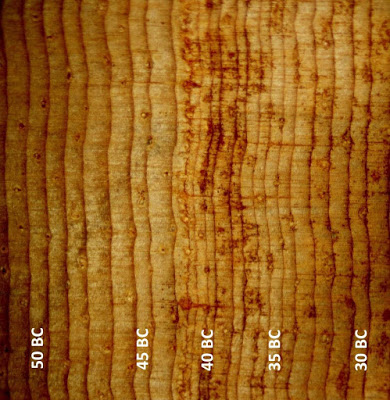
Narrow and distorted tree-rings from long living bristlecone-pines (Snake Mountains, Nevada, USA), indicating extreme cooling after a large volcanic eruption in 44 BCE, the year of Julius Cesar’s death. Credit: Matthew Salzer
It is well known that large volcanic eruptions contribute to climate variability. However, quantifying these contributions has proven challenging due to inconsistencies in both historic atmospheric data observed in ice cores and corresponding temperature variations seen in climate proxies such as tree rings.
Published today in the journal Nature, a new study led by scientists from the Desert Research Institute (DRI) and collaborating international institutions, resolves these inconsistencies with a new reconstruction of the timing and associated radiative forcing of nearly 300 individual volcanic eruptions extending as far back as the early Roman period.
“Using new records we are able to show that large volcanic eruptions in the tropics and high latitudes were the dominant drivers of climate variability, responsible for numerous and widespread summer cooling extremes over the past 2,500 years,” said the study’s lead author Michael Sigl, Ph.D., an assistant research professor at DRI and postdoctoral fellow with the Paul Scherrer Institute in Switzerland.
“These cooler temperatures were caused by large amounts of volcanic sulfate particles injected into the upper atmosphere,” Sigl added, “shielding the Earth’s surface from incoming solar radiation.”
The study shows that 15 of the 16 coldest summers recorded between 500 BC and 1,000 AD followed large volcanic eruptions — with four of the coldest occurring shortly after the largest volcanic events found in record.
This new reconstruction is derived from more than 20 individual ice cores extracted from ice sheets in Greenland and Antarctica and analyzed for volcanic sulfate primarily using DRI’s state-of-the-art, ultra-trace chemical ice-core analytical system.
These ice-core records provide a year-by-year history of atmospheric sulfate levels through time. Additional measurements including other chemical parameters were made at collaborating institutions.
“We used a new method for producing the timescale,” explained Mai Winstrup, Ph.D., a postdoctoral researcher at the University of Washington, Seattle. “Previously, this has been done by hand, but we used a statistical algorithm instead. Together with the state-of-the-art ice core chemistry measurements, this resulted in a more accurate dating of the ice cores.”
“Using a multidisciplinary approach was key to the success of this project,” added Sigl.
In total, a diverse research group of 24 scientists from 18 universities and research institutes in the United States, United Kingdom, Switzerland, Germany, Denmark, and Sweden contributed to this work — including specialists from the solar, space, climate, and geological sciences, as well as historians.
The authors note that identification of new evidence found in both ice cores and corresponding tree rings allowed constraints and verification of their new age scale.
“With the discovery of a distinctive signature in the ice-core records from an extra-terrestrial cosmic ray event, we had a critical time marker that we used to significantly improve the dating accuracy of the ice-core chronologies,” explained Kees Welten, Ph.D., an associate research chemist from the University of California, Berkeley.
A signature from this same event had been identified earlier in various tree-ring chronologies dating to 774-775 Common Era (CE).
“Ice-core timescales had been misdated previously by five to ten years during the first millennium leading to inconsistencies in the proposed timing of volcanic eruptions relative to written documentary and tree-ring evidence recording the climatic responses to the same eruptions,” explained Francis Ludlow, Ph.D., a postdoctoral fellow from the Yale Climate & Energy Institute.
Throughout human history, sustained volcanic cooling effects on climate have triggered crop failures and famines. These events may have also contributed to pandemics and societal decline in agriculture-based communities.
Together with Conor Kostick, Ph.D. from the University of Nottingham, Ludlow translated and interpreted ancient and medieval documentary records from China, Babylon (Iraq), and Europe that described unusual atmospheric observations as early as 254 years before Common Era (BCE). These phenomena included diminished sunlight, discoloration of the solar disk, the presence of solar coronae, and deeply red twilight skies.
Tropical volcanoes and large eruptions in the Northern Hemisphere high latitudes (such as Iceland and North America) — in 536, 626, and 939 CE, for example — often caused severe and widespread summer cooling in the Northern Hemisphere by injecting sulfate and ash into the high atmosphere. These particles also dimmed the atmosphere over Europe to such an extent that the effect was noted and recorded in independent archives by numerous historical eyewitnesses.
Climatic impact was strongest and most persistent after clusters of two or more large eruptions.
The authors note that their findings also resolve a long-standing debate regarding the causes of one of the most severe climate crises in recent human history, starting with an 18-month “mystery cloud” or dust veil observed in the Mediterranean region beginning in March, 536, the product of a large eruption in the high-latitudes of the Northern Hemisphere.
The initial cooling was intensified when a second volcano located somewhere in the tropics erupted only four years later. In the aftermath, exceptionally cold summers were observed throughout the Northern Hemisphere.
This pattern persisted for almost fifteen years, with subsequent crop failures and famines — likely contributing to the outbreak of the Justinian plague that spread throughout the Eastern Roman Empire from 541 to 543 CE, and which ultimately decimated the human population across Eurasia.
“This new reconstruction of volcanic forcing will lead to improved climate model simulations through better quantification of the sensitivity of the climate system to volcanic influences during the past 2,500 years,” noted Joe McConnell, Ph.D., a DRI research professor who developed the continuous-flow analysis system used to analyze the ice cores.
“As a result,” McConnell added, “climate variability observed during more recent times can be put into a multi-millennial perspective — including time periods such as the Roman Warm Period and the times of significant cultural change such as Great Migration Period of the 6th century in Europe.”
This reconciliation of ice-core records and other records of past environmental change will help define the role that large climatic perturbations may have had in the rise and fall of civilizations throughout human history.
“With new high-resolution records emerging from ice cores in Greenland and Antarctica, it will be possible to extend this reconstruction of volcanic forcing probably all the way back into the last Ice Age,” said Sigl.
This research was largely funded by the U.S. National Science Foundation’s Polar Program; with contributions from additional funding agencies and institutions in Belgium, Canada, China, Denmark, France, Germany, Iceland, Japan, Korea, The Netherlands, Sweden, Switzerland, and the United Kingdom.
Reference:
M. Sigl, M. Winstrup, J. R. McConnell, K. C. Welten, G. Plunkett, F. Ludlow, U. Büntgen, M. Caffee, N. Chellman, D. Dahl-Jensen, H. Fischer, S. Kipfstuhl, C. Kostick, O. J. Maselli, F. Mekhaldi, R. Mulvaney, R. Muscheler, D. R. Pasteris, J. R. Pilcher, M. Salzer, S. Schüpbach, J. P. Steffensen, B. M. Vinther, T. E. Woodruff. Timing and climate forcing of volcanic eruptions for the past 2,500 years. Nature, 2015; DOI: 10.1038/nature14565
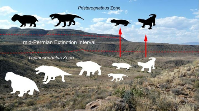
This is an illustration of the Guadalupian extinction. Credit: Wits University
An international team led by researchers from the Evolutionary Studies Institute (ESI) at the University of the Witwatersrand, Johannesburg, has obtained an age from rocks of the Great Karoo that shed light on the timing of a mass extinction event that occurred around 260 million years ago.
This led to the disappearance of a diverse group of early mammal-like reptiles called dinocephalians, which were the largest land-living animals of the time.
The project was led by Dr Michael Day, a postdoctoral fellow at Wits University, and the findings are contained in paper, titled: When and how did the terrestrial mid-Permian mass extinction occur? Evidence from the tetrapod record of the Karoo Basin, South Africa, published today, 8 July 2015, in the latest issue of the Royal Society’s biological journal, Proceedings of the Royal Society B.
The Karoo is very rich in fossils of terrestrial animals from the Permian and Triassic geological periods, which makes it one of the few places to study extinction events on land during this time. As a result South Africa’s Karoo region provides not only a historical record of biological change over a period of Earth’s history but also a means to test theories of evolutionary processes over long stretches of time.
By collecting fossils in the Eastern, Western and Northern Cape Provinces the team was able to show that around 74-80% of species became extinct along with the dinocephalians in a geologically short period of time.
The new date was obtained by high precision analyses of the relative abundance of uranium and lead in small zircon crystals from a volcanic ash layer close to this extinction horizon in the Karoo.
This provides a means of linking the South African fossil record with the fossil record in the rest of the world. In particular, it helps correlate the Karoo with the global marine record, which also records an extinction event around 260 million years ago.
“A mid-Permian extinction event on land has been known for some time but was suspected to have occurred earlier than those in the marine realm. The new date suggests that one event may have affected marine and terrestrial environments at the same time, which could mean its impact was greater than we thought,” says Day.
The mid-Permian extinction occurred near the end of what geologists call the Guadalupian epoch that extended from 272.3 to around 259.1 million years ago. It pre-dated the massive and much more famous end-Permian mass extinction event by 8 million years.
“The South African Karoo rocks host the richest record of middle Permian land-living vertebrate animals. This dataset, the culmination of 30 years of fossil collecting and diligent stratigraphic recording of the information, for the first time provides robust fossil and radioisotopic data to support the occurrence of this extinction event on land,” says Day.
“The exact age of the marine extinctions remains uncertain,” says Jahandar Ramezani of Massachusetts Institute of Technology and who was responsible for dating the rocks, “but this new date from terrestrial deposits of the Karoo, supported by palaeontological evidence, represents an important step towards a better understanding of the mid-Permian extinction and its effect on terrestrial faunas.”
Reference:
Michael O. Day, Jahandar Ramezani, Samuel A. Bowring, Peter M. Sadler, Douglas H. Erwin, Fernando Abdala, Bruce S. Rubidge. When and how did the terrestrial mid-Permian mass extinction occur? Evidence from the tetrapod record of the Karoo Basin, South Africa. Proceedings of the Royal Society B, 2015 DOI: 10.1098/rspb.2015.0834
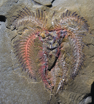
A marrellomorph arthropod, probably belonging to the genus Furca. c. Credit: Peter Van Roy
Some of the oldest marine animals on the planet, including armoured worm-like forms and giant, lobster like sea creatures, survived millions of years longer than previously thought, according to a spectacularly preserved fossil formation from southeastern Morocco.
The Lower Fezouata formation has been revealing exciting discoveries about life in the Ordovician — around 485 — 444 million years ago — since its discovery just five years ago.
‘The Fezouata is extraordinarily significant’ says Professor Derek Briggs of Yale University, co-author of a study published today in the Journal of the Geological Society. ‘Animals typical of the Cambrian are still present in rocks 20 million years younger, which means there must be a cryptic record in between, which is not preserved.’
Over 160 genera have already been documented from the Fezouata, with much more expected to be found. They include animals which would have looked perfectly at home during the Cambrian: armoured lobopodians — worm like creatures with spines on their backs and short, stubby legs, and anomalocaridids — huge segmented animals with remarkable feeding limbs, which are some of the largest marine creatures of the time.
As well as demonstrating the longevity of fauna thought to have been extinct millions of years previously, the Fezouata proves that other creatures evolved far earlier than previously thought.
‘Horseshoe crabs, for example, turn out to be at least 20 million years older than we thought. The formation demonstrates how important exceptionally preserved fossils are to our understanding of major evolutionary events in deep time’ says Peter Van Roy, also of Yale, who first recognised the scientific importance of the Fezouata fauna and is lead author of the study, part of a project funded by the National Science Foundation.
The spectacular preservation, which includes detailed soft parts and organisms over 2 metres in length, is thanks to the fine grained, muddy sediments in which the organisms were preserved.
‘These are special rocks’ says Professor Briggs. ‘Some of the organisms are enormous — several metres in length. With such exceptional preservation, in a fully marine exposure, we can develop a reasonably full picture of what marine life looked like in the Ordovician.’
The discoveries suggest the ‘Great Ordovician Biodiversification Event’ — an explosion in diversity throughout the earlier part of the Ordovician period — may have been a continuation of the Cambrian explosion.
‘There is much more to learn from the Fezouata’ says Professor Briggs. ‘Why do we not see more assemblages like this in the Ordovician? What ecological changes happened at the Cambro-Ordovician interval? Are the Cambrian Explosion and the Great Ordovician Biodiversification Event separate, or phases of the same event?’
The paper, published online today, marks the start of a themed series of ‘Review focus’ articles for the Journal of the Geological Society, centring on sites of exceptional fossil preservation spanning Earth’s history. All papers in the series will be available for free download, and further ‘Review focus’ themes are planned.
‘The purpose of these articles is to present a distilled, forward looking review of a topic’, says the series editor Professor Philip Donoghue. ‘We decided to start with a thematic series on fossil Lagerstätten since these deposits are fundamental archives of evolutionary history.’
‘By making the papers freely available, it is hoped they will interest a wide range of readers, from undergraduates, to specialists in the field, to members of the public.’
Reference:
Van Roy, P., Briggs, D.E.G. & Gaines R.R. The Fezouata fossils of Morocco; an extraordinary record of marine life in the Early Ordovician. Journal of the Geological Society, July 8, 2015 DOI: 10.1144/jgs2015-017
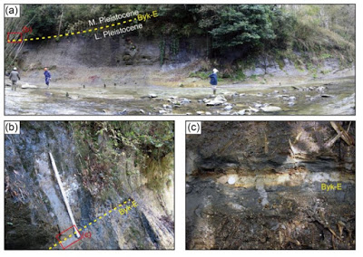
This is a photograph of the geological section across the Matuyama-Brunhes boundary in Chiba Prefecture, Japan. (a) Overview of the Chiba section. (b) and (c) Detail of a volcanic ash layer (Byk-E) just below the MBB in the Chiba section. The length of the ruler (b) and diameter of the coin (c) are 1.25 m and 2 cm, respectively. Credit: NIPR/Ibaraki University/JAMSTEC
Earth’s magnetic field periodically reverses such that the north magnetic pole becomes the south magnetic pole. The latest reversal is called by geologists the Matuyama-Brunhes boundary (MBB), and occurred approximately 780,000 years ago. The MBB is extremely important for calibrating the ages of rocks and the timing of events that occurred in the geological past; however, the exact age of this event has been imprecise because of uncertainties in the dating methods that have been used.
A team of researchers based in Japan and Canada have obtained an improved age for the MBB. The team studied volcanic ash that was deposited immediately before the MBB. This volcanic ash contains small crystals called zircons. Some of these crystals formed at the same time as the ash; thus, radiometric dating of these zircons using the uranium-lead method provided the exact age of the ash. To verify their findings, the researchers also used a different method to date sedimentary rock from the same place that was formed at the time of the MBB. The combined results demonstrate that the age of the MBB is 770.2 ± 7.3 thousand years ago. The research has been published in the journal Geology.
Dr. Yusuke Suganuma of the National Institute of Polar Research, Tokyo, who is the lead author on the paper, commented: “This study is the first direct comparison of radiometric dating, dating of sediments, and the geomagnetic reversal for the Matuyama-Brunhes boundary. Our work contributes calibrating the geological time scale, and will be extremely important in future studies of the events that occurred at this time.”
Reference:
Y. Suganuma, M. Okada, K. Horie, H. Kaiden, M. Takehara, R. Senda, J.-I. Kimura, K. Kawamura, Y. Haneda, O. Kazaoka, M. J. Head. Age of Matuyama-Brunhes boundary constrained by U-Pb zircon dating of a widespread tephra. Geology, 2015; 43 (6): 491 DOI: 10.1130/G36625.1
Although global concentration of greenhouse gases in the atmosphere has continuously increased over the past decade, the mean global surface temperature has not followed the same path. A team of international reseachers, KIT scientists among them, have now found an explanation for this slowing down in global warming: the incoming solar radiation in the years 2008-2011 was twice as much reflected by volcanic aerosol particles in the lowest part of the stratosphere than previously thought. The team presents their study in Nature Communications.
For the lowest part of the stratosphere – i. e. the layer between 10 and 16 kilometres – little information was available so far, but now the international IAGOS-CARIBIC climate project combined with satellite observations from the CALIPSO lidar provided new essential information. According to the study, the cooling effect due to volcanic eruptions was clearly underestimated by climate models used for the last Intergovernmental Panel on Climate Change (IPCC) report. Led by the University of Lund, Sweden, and supported by the NASA Langley Research Center, USA, and the Royal Netherlands Meteorological Institute, three major German atmospheric research institutes were also involved: the Max Planck Institute for Chemistry in Mainz (MPI-C), the Leibniz Institute for Tropospheric Research in Leipzig (TROPOS) and the Karlsruhe Institute of Technology (KIT). Since more frequent volcanic eruptions and the subsequent cooling effect are only temporary the rise of Earths’ temperature will speed up again. The reason is the still continuously increasing greenhouse gas concentration, the scientists say.
In the first decade of the 21st century the average surface temperature over the northern mid-latitude continents did increase only slightly. This effect can be now explained by the new study on volcanic aerosol particles in the atmosphere reported here. The study uses data from the tropopause region up to 35 km altitude, where the former is found between 8 km (poles) and 17 km (equator) altitude. The tropopause region is a transition layer between the underlying wet weather layer with its clouds (troposphere) and the dry and cloud-free layer above (stratosphere). “Overall our results emphasize that even smaller volcanic eruptions are more important for the Earth´s climate than expected”, summarize CARIBIC coordinators Dr. Carl Brenninkmeijer, MPI-C, and Dr. Andreas Zahn, KIT. The IAGOS-CARIBIC observatory was coordinated and operated by the MPI-C until the end of 2014, since then by the KIT.
To collect their data the team combined two different experimental approaches: sampling and in situ measurements made by IAGOS-CARIBIC together with observations from the CALIPSO satellite. In the IAGOS-CARIBIC observatory trace gases and aerosol particles in the tropopause region are measured since 1997. A modified air-freight container is loaded once per month for four intercontinental flights into a modified Airbus A340-600 of Lufthansa. Altogether about 100 trace gas and aerosol parameters are measured in situ at 9-12 km altitude as well as in dedicated European research laboratories after flight. TROPOS in Leipzig is responsible for the in situ aerosol particle measurements in this unique project. KIT runs 5 of the 15 installed instruments, also the one for ozone. Collected particles are analyzed at the University of Lund, Sweden, using an ion beam accelerator for measuring the amount of particulate sulfur. When comparing this particulate sulfur concentration to the in situ measured ozone concentration this ratio is usually quite constant at cruise altitude. However, volcanic eruptions increase the amount of particulate sulfur and thus the ratio becomes an indicator of volcanic eruption influencing the tropopause region. “The ratio of particulate sulfur to ozone from the CARIBIC measurements clearly demonstrates the strong influence from volcanism on the tropopause region”, report Dr. Sandra M. Andersson and Professor Bengt G. Martinsson of the University of Lund, who are the lead authors.
The second method is based on satellite observations. The Cloud-Aerosol Lidar and Pathfinder Satellite Observation (CALIPSO) mission, a collaboration between the National Aeronautics and Space Administration (NASA) in the US and the Centre National d’Etude Spatiale (CNES) in France, has provided unprecedented view on aerosol and cloud layers in the atmosphere. Until recently, the data had only been scrutinized above 15 km, namely where volcanic aerosol are known to affect our climate for a long time. Now also aeorosol particles of the lowermost stratosphere have been taken into account for calculating the radiative balance of the atmosphere, to evaluate the impact of smaller volcanic eruptions on the climate.
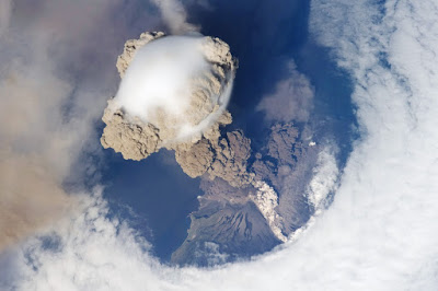
The influence from volcanic eruptions on the stratosphere was small in the northern hemisphere between 1999 and 2002. However, strong signals of volcanic aerosol particles were observed between 2005 and 2012. In particular three eruptions stand out: the Kasatochi in August 2008 (USA), the Sarychev in June 2009 (Russia), and the Nabro in June 2011 (Eritrea). Each of the three eruptions injected more than one megaton sulfur dioxide (SO2) into the atmosphere. “Virtually all volcanic eruptions reaching the stratosphere lead to more particles there, as they bring in sulfur dioxide, which is converted to sulfate particles”, explains Dr. Markus Hermann of TROPOS, who conducts the in situ particle measurements in CARIBIC.
Whether a volcanic eruption has a global climate impact or not depends on several factors. There is the amount of volcanic sulfur dioxide as well as the injection height. But also the latitude of the eruption is important: As the air flow in northern hemispheric stratosphere is largely disconnected from the southern hemisphere, only volcanic eruptions near the equator can effectively distribute the emitted material over both hemispheres. As in the Tambora eruption on the Indonesian Island Sumbawa 200 years ago. This eruption led to such a strong global cooling that the year 1816 was called “year without summer”, including worldwide crop failures and famines. Also the Krakatau eruption 1883 on Indonesia or the Pinatubo 1991 on the Philippines led to noticeable cooling. The present study now indicates that “the cooling effect of volcanic eruptions was underestimated in the past, because the lowest part of the stratosphere was mostly not considered. Interestingly our results show that the effect also depends on the season. The eruptions investigated by us had their strongest impact in late summer when the incoming solar radiation is still strong”, explains Dr. Sandra M. Andersson.
Reference:
“Significant radiative impact of volcanic aerosol in the lowermost stratosphere.” Nature Communications, DOI: 10.1038/ncomms8692
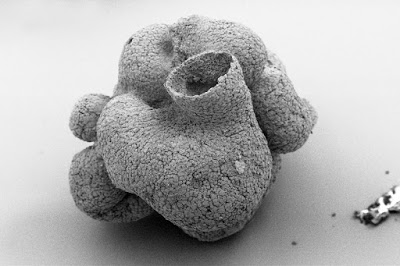
The tiny fossil sponge was just 1.2 millimeters in width, seen here in a high-resolution scanning electron microscope image. Credit: Zongjun Yin/Nanjing Institute of Geology and Palaeontology
Researchers have unearthed a fossil of a sponge, no bigger than a grain of sand, that existed 60 million years earlier than many expected.
This is the first time paleontologists have found a convincing fossil sponge specimen that predates the Cambrian explosion—a 20-million-year phenomenon, beginning about 542 million years ago, when most major types of animal life appear.
New tools could allow scientists to discover other fossils that significantly predate the start of the Cambrian explosion, according to David Bottjer, professor of earth sciences, biological sciences and environmental studies and co-author of a study announcing the finding of the sponge in the Proceedings of the National Academy of Sciences.
“It’s easier to look at large fossils that don’t require high-tech instruments,” Bottjer said. “We’re analyzing very tiny things that require sophisticated microscopy, and we’re really just starting to look at this kind of evidence.”
Preserved fossils
Though some evidence, including molecular clocks, has already pointed to sponges evolving earlier, this fossil shows that the Cambrian explosion might not be a period when a large number of new traits emerged, but a period when a large number of fossils could be preserved, as animals during the Cambrian grew larger and gained skeletons.
“This specimen is of an animal that had already evolved a number of fundamental sponge traits,” Bottjer said. “It implies that by the time this animal was living, most of the developmental genes for sponges had evolved.”
This raises the possibility that some aspects of early animals’ evolution, a good deal of which happened during the Cambrian explosion, happened even more gradually.
With an international team of colleagues, Bottjer discovered that the millimeter-wide, 600-million-year-old fossil has characteristics that many thought emerged in sponges only 540 million years ago.
“Fundamental traits in sponges were not suddenly appearing in the Cambrian Period, which is when many think these traits were evolving, but many million years earlier,” Bottjer said. “To reveal these types of findings, you have to use pretty high-tech approaches and work with the best people around the world.”
Very old rocks
Since 1999, Bottjer has worked with a team of researchers from the Nanjing Institute of Geology and Palaeontology (Chinese Academy of Sciences) and the California Institute of Technology, as well as the European Synchrotron Radiation Facility in Grenoble, France.
Team members in China dissolved several 600 million-year-old rocks, which are regularly mined for Chinese agricultural fertilizer from the Doushantuo rock formation in southwestern China’s Guizhou Province. They then used a gentle acid bath to reveal tiny fossils made of calcium phosphate and a Scanning Electron Microscope (SEM) to determine which of those fossils were preserved well enough to merit analysis with the synchrotron.
“The preservation in these Doushantuo rocks is extremely fine—and you can even see individual cells with the SEM,” Bottjer said. “Once a specimen worthy of further study is found, synchrotron microscopy is used to create very, very detailed images of the fossil in two and three dimensions. From these images we are then able to see what types of animals these fossils represent.”
Future study lies in the relatively new field of paleogenomics, which analyzes the evolutionary history of genes to determine when individual genes first appeared. Bottjer said many of the genes operating in sponges 600 million years ago are the same genes that other animals have, including humans.
“These organisms don’t have all the bells and whistles that modern creatures do,” Bottjer said. “But this particular fossil has enough complexity that we can say we hadn’t been dating the early evolution of animal traits properly.”
A) Skull of the therapsid Pristerodon; B) Image obtained from neutron tomographic data. Credit: Image courtesy of the author.
A recent study by means of neutron tomography revealed that some forerunners of mammals were already able to hear airborne sound, because these animals already possessed an eardrum at the lower jaw, an impedance-matching middle ear and a small cochlea.
Most land animals can only hear sound from the air via a specialised area for sound reception – the eardrum. Furthermore, the middle ear consisting of three ear ossicles, the malleus, incus and stapes, amplifies sound impulses from the eardrum, and the cochlea is responsible for transforming a wide range of sound frequencies into nerve impulses for the brain.
In contrast, early land-living tetrapods were originally unable to hear airborne sound, because they evolved from aquatic ancestors. Instead, it seems likely that they could only detect seismic sound from the ground with the mandible, like some modern snakes. Until recently, it was unresolved whether the forerunners of mammals, the therapsids, already possessed an eardrum and an impedance-matching middle ear to hear sound from the air or not.
Interestingly, it was discovered almost 200 years ago that the mammalian ear ossicles are the homologues of the the articular and quadrate, the bones that form the jaw articulation in reptiles and in the forerunners of mammals. In early mammalian evolution, a new jaw articulation evolved and these bones were separated from the skull and the mandible and only served for hearing. Therefore, it was uncertain if therapsids were already able to hear airborne sound. If so, their massive jaw articulation must have had a dual function – to withstand the forces from feeding and to conduct weak sound impulses to the inner ear.
To shed light on this problem, Michael Laaß from the University of Duisburg-Essen investigated a ca. 260 million years old skull of the therapsid Pristerodon from the Karoo Basin of South Africa by means of neutron tomography. The experiments were conducted at the Swiss spallation neutron source SINQ, Paul Scherrer Institute in Switzerland, and were supported through the NMI3 Access Programme.
As stated by Laaß “Neutron tomography was well suited to investigate the skull because neutrons were able to penetrate this fossil very well and produce a good contrast between the fossil bones and the matrix.” This investigation revealed the earliest evidence of a cochlea in a far relative of mammals. Moreover, it was possible to reconstruct the ear virtually in 3D and to reconstruct the function of the middle ear. Interestingly, the latter was able to amplify sound and to conduct weak sound impulses from the mandible to the inner ear if the jaw musculature was relaxed.
Furthermore, the postcranial anatomy of Pristerodon suggests that this animal already had a more upright posture than other therapsids. As a consequence, the lower jaw was usually not in contact with the ground and hearing of seismic sound was impossible. This might be the reason why Pristerodon evolved an airborne-sound-sensitive ear, because this was necessary to detect predators or to communicate with conspecifics.
Reference:
Laaß, Michael. 2015. “The origins of the cochlea and impedance matching hearing in synapsids.” Acta Palaeontologica Polonica. DOI: 10.4202/app.00140.2014
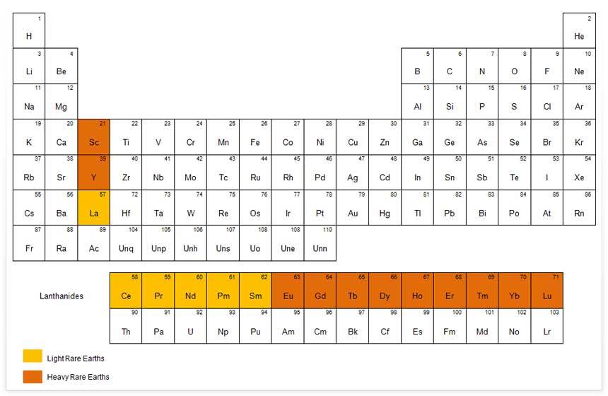
A rare earth element (REE) or rare earth metal (REM), as defined by IUPAC, is one of a set of seventeen chemical elements in the periodic table, specifically the fifteen lanthanides, as well as scandium and yttrium. Scandium and yttrium are considered rare earth elements because they tend to occur in the same ore deposits as the lanthanides and exhibit similar chemical properties.
Despite their name, rare earth elements are – with the exception of the radioactive promethium – relatively plentiful in Earth’s crust, with cerium being the 25th most abundant element at 68 parts per million, or as abundant as copper. However, because of their geochemical properties, rare earth elements are typically dispersed and not often found concentrated as rare earth minerals in economically exploitable ore deposits. It was the very scarcity of these minerals (previously called “earths”) that led to the term “rare earth”. The first such mineral discovered was gadolinite, a mineral composed of cerium, yttrium, iron, silicon and other elements. This mineral was extracted from a mine in the village of Ytterby in Sweden; four of the rare earth elements bear names derived from this single location.
Discovery and early history
Rare earth elements became known to the world with the discovery of the black mineral “Ytterbite” (renamed to Gadolinite in 1800) by Lieutenant Carl Axel Arrhenius in 1787, at a quarry in the village of Ytterby, Sweden.
Arrhenius’s “ytterbite” reached Johan Gadolin, a Royal Academy of Turku professor, and his analysis yielded an unknown oxide (earth) that he called yttria. Anders Gustav Ekeberg isolated beryllium from the gadolinite but failed to recognize other elements that the ore contained. After this discovery in 1794 a mineral from Bastnäs near Riddarhyttan, Sweden, which was believed to be an iron–tungsten mineral, was re-examined by Jöns Jacob Berzelius and Wilhelm Hisinger. In 1803 they obtained a white oxide and called it ceria. Martin Heinrich Klaproth independently discovered the same oxide and called it ochroia.
Thus by 1803 there were two known rare earth elements, yttrium and cerium, although it took another 30 years for researchers to determine that other elements were contained in the two ores ceria and yttria (the similarity of the rare earth metals’ chemical properties made their separation difficult).
In 1839 Carl Gustav Mosander, an assistant of Berzelius, separated ceria by heating the nitrate and dissolving the product in nitric acid. He called the oxide of the soluble salt lanthana. It took him three more years to separate the lanthana further into didymia and pure lanthana. Didymia, although not further separable by Mosander’s techniques, was a mixture of oxides.
In 1842 Mosander also separated the yttria into three oxides: pure yttria, terbia and erbia (all the names are derived from the town name “Ytterby”). The earth giving pink salts he called terbium; the one that yielded yellow peroxide he called erbium.
So in 1842 the number of known rare earth elements had reached six: yttrium, cerium, lanthanum, didymium, erbium and terbium.
Nils Johan Berlin and Marc Delafontaine tried also to separate the crude yttria and found the same substances that Mosander obtained, but Berlin named (1860) the substance giving pink salts erbium and Delafontaine named the substance with the yellow peroxide terbium. This confusion led to several false claims of new elements, such as the mosandrium of J. Lawrence Smith, or the philippium and decipium of Delafontaine.
Origin
Rare earth elements, except scandium, are heavier than iron and thus are produced by supernova nucleosynthesis or the s-process in asymptotic giant branch stars. In nature, spontaneous fission of uranium-238 produces trace amounts of radioactive promethium, but most promethium is synthetically produced in nuclear reactors.
Rare earth elements change through time in small quantities (ppm, parts per million), so their proportion can be used for geochronology and dating fossils.
Geological distribution
Rare earth cerium is actually the 25th most abundant element in Earth’s crust, having 68 parts per million (about as common as copper). Only the highly unstable and radioactive promethium “rare earth” is quite scarce.
The rare earth elements are often found together. The longest-lived isotope of promethium has a half life of 17.7 years, so the element exists in nature in only negligible amounts (approximately 572 g in the entire Earth’s crust). Promethium is one of the two elements that do not have stable (non-radioactive) isotopes and are followed by (i.e. with higher atomic number) stable elements (the other being technetium).
Due to lanthanide contraction, yttrium, which is trivalent, is of similar ionic size as dysprosium and its lanthanide neighbors. Due to the relatively gradual decrease in ionic size with increasing atomic number, the rare earth elements have always been difficult to separate. Even with eons of geological time, geochemical separation of the lanthanides has only rarely progressed much farther than a broad separation between light versus heavy lanthanides, otherwise known as the cerium and yttrium earths. This geochemical divide is reflected in the first two rare earths that were discovered, yttria in 1794 and ceria in 1803. As originally found, each comprised the entire mixture of the associated earths. Rare earth minerals, as found, usually are dominated by one group or the other, depending on which size range best fits the structural lattice.
Thus, among the anhydrous rare earth phosphates, it is the tetragonal mineral xenotime that incorporates yttrium and the yttrium earths, whereas the monoclinic monazite phase incorporates cerium and the cerium earths preferentially. The smaller size of the yttrium group allows it a greater solid solubility in the rock-forming minerals that comprise Earth’s mantle, and thus yttrium and the yttrium earths show less enrichment in Earth’s crust relative to chondritic abundance, than does cerium and the cerium earths. This has economic consequences: large ore bodies of the cerium earths are known around the world, and are being exploited. Corresponding orebodies for yttrium tend to be rarer, smaller, and less concentrated. Most of the current supply of yttrium originates in the “ion absorption clay” ores of Southern China. Some versions provide concentrates containing about 65% yttrium oxide, with the heavy lanthanides being present in ratios reflecting the Oddo-Harkins rule: even-numbered heavy lanthanides at abundances of about 5% each, and odd-numbered lanthanides at abundances of about 1% each. Similar compositions are found in xenotime or gadolinite.
Well-known minerals containing yttrium include gadolinite, xenotime, samarskite, euxenite, fergusonite, yttrotantalite, yttrotungstite, yttrofluorite (a variety of fluorite), thalenite, yttrialite. Small amounts occur in zircon, which derives its typical yellow fluorescence from some of the accompanying heavy lanthanides. The zirconium mineral eudialyte, such as is found in southern Greenland, contains small but potentially useful amounts of yttrium. Of the above yttrium minerals, most played a part in providing research quantities of lanthanides during the discovery days. Xenotime is occasionally recovered as a byproduct of heavy sand processing, but is not as abundant as the similarly recovered monazite (which typically contains a few percent of yttrium). Uranium ores from Ontario have occasionally yielded yttrium as a byproduct.
Well-known minerals containing cerium and the light lanthanides include bastnäsite, monazite, allanite, loparite, ancylite, parisite, lanthanite, chevkinite, cerite, stillwellite, britholite, fluocerite, and cerianite. Monazite (marine sands from Brazil, India, or Australia; rock from South Africa), bastnäsite (from Mountain Pass, California, or several localities in China), and loparite (Kola Peninsula, Russia) have been the principal ores of cerium and the light lanthanides.
In 2011, Yasuhiro Kato, a geologist at the University of Tokyo who led a study of Pacific Ocean seabed mud, published results indicating the mud could hold rich concentrations of rare earth minerals. The deposits, studied at 78 sites, came from “[h]ot plumes from hydrothermal vents pull[ing] these materials out of seawater and deposit[ing] them on the seafloor, bit by bit, over tens of millions of years. One square patch of metal-rich mud 2.3 kilometers wide might contain enough rare earths to meet most of the global demand for a year, Japanese geologists report July 3 in Nature Geoscience.” “I believe that rare earth resources undersea are much more promising than on-land resources,” said Kato. “[C]oncentrations of rare earths were comparable to those found in clays mined in China. Some deposits contained twice as much heavy rare earths such as dysprosium, a component of magnets in hybrid car motors.”
Global rare earth production
Until 1948, most of the world’s rare earths were sourced from placer sand deposits in India and Brazil. Through the 1950s, South Africa took the status as the world’s rare earth source, after large veins of rare earth bearing monazite were discovered there. Through the 1960s until the 1980s, the Mountain Pass rare earth mine in California was the leading producer. Today, the Indian and South African deposits still produce some rare earth concentrates, but they are dwarfed by the scale of Chinese production. In 2010, China produced over 95% of the world’s rare earth supply, mostly in Inner Mongolia, although it had only 37% of proven reserves; the latter number has been reported to be only 23% in 2012. All of the world’s heavy rare earths (such as dysprosium) come from Chinese rare earth sources such as the polymetallic Bayan Obo deposit. In 2010, the United States Geological Survey (USGS) released a study that found that the United States had 13 million metric tons of rare earth elements.
New demand has recently strained supply, and there is growing concern that the world may soon face a shortage of the rare earths. In several years from 2009 worldwide demand for rare earth elements is expected to exceed supply by 40,000 tonnes annually unless major new sources are developed.
Global rare earth element production from 1950 through 2000, colored to indicate source. (1 kt=106 kg) Credit: BMacZero
Rare earth pricing
Rare earth elements are not exchange-traded in the same way that precious (for instance, gold and silver) or non-ferrous metals (such as nickel, tin, copper, and aluminium) are. Instead they are sold on the private market, which makes their prices difficult to monitor and track. The 17 elements are not usually sold in their pure form, but instead are distributed in mixtures of varying purity, e.g. “Neodymium metal ≥ 99%”. As such, pricing can vary based on the quantity and quality required by the end user’s application.
Oil sands, Tar sands or, more technically, bituminous sands, are a type of unconventional petroleum deposit.
Oil sands are either loose sands or partially consolidated sandstone containing a naturally occurring mixture of sand, clay, and water, saturated with a dense and extremely viscous form of petroleum technically referred to as bitumen (or colloquially tar due to its similar appearance, odour, and colour). Natural bitumen deposits are reported in many countries, but in particular are found in extremely large quantities in Canada. Other large reserves are located in Kazakhstan and Russia. The estimated worldwide deposits of oil are more than 2 trillion barrels (320 billion cubic metres); the estimates include deposits that have not been discovered. Proven reserves of bitumen contain approximately 100 billion barrels, and total natural bitumen reserves are estimated at 249.67 Gbbl (39.694×10⁹ m3) worldwide, of which 176.8 Gbbl (28.11×10⁹ m3), or 70.8%, are in Alberta, Canada.
Oil sands reserves have only recently been considered to be part of the world’s oil reserves, as higher oil prices and new technology enable profitable extraction and processing. Oil produced from bitumen sands is often referred to as unconventional oil or crude bitumen, to distinguish it from liquid hydrocarbons produced from traditional oil wells.
The crude bitumen contained in the Canadian oil sands is described by the National Energy Board of Canada as “a highly viscous mixture of hydrocarbons heavier than pentanes which, in its natural state, is not usually recoverable at a commercial rate through a well because it is too thick to flow.” Crude bitumen is a thick, sticky form of crude oil, so heavy and viscous (thick) that it will not flow unless heated or diluted with lighter hydrocarbons such as light crude oil or natural-gas condensate. At room temperature, it is much like cold molasses. The World Energy Council (WEC) defines natural bitumen as “oil having a viscosity greater than 10,000 centipoise under reservoir conditions and an API gravity of less than 10° API”. The Orinoco Belt in Venezuela is sometimes described as oil sands, but these deposits are non-bituminous, falling instead into the category of heavy or extra-heavy oil due to their lower viscosity. Natural bitumen and extra-heavy oil differ in the degree by which they have been degraded from the original conventional oils by bacteria. According to the WEC, extra-heavy oil has “a gravity of less than 10° API and a reservoir viscosity of no more than 10,000 centipoise”.
Tar sandstone from the Monterey Formation of Miocene age (10 to 12 million years old), of southern California, USA. Credit: James St. John
According to the study ordered by the Government of Alberta and conducted by Jacobs Engineering Group, emissions from oil-sand crude are 12% higher than from conventional oil.
History
The exploitation of bituminous deposits and seeps dates back to Paleolithic times. The earliest known use of bitumen was by Neanderthals, some 40,000 years ago. Bitumen has been found adhering to stone tools used by Neanderthals at sites in Syria. After the arrival of Homo sapiens, humans used bitumen for construction of buildings and waterproofing of reed boats, among other uses. In ancient Egypt, the use of bitumen was important in preparing Egyptian mummies.
In ancient times, bitumen was primarily a Mesopotamian commodity used by the Sumerians and Babylonians, although it was also found in the Levant and Persia. The area along the Tigris and Euphrates rivers was littered with hundreds of pure bitumen seepages. The Mesopotamians used the bitumen for waterproofing boats and buildings. In Europe, they were extensively mined near the French city of Pechelbronn, where the vapour separation process was in use in 1742.
Nomenclature
The name tar sands was applied to bituminous sands in the late 19th and early 20th century. People who saw the bituminous sands during this period were familiar with the large amounts of tar residue produced in urban areas as a by-product of the manufacture of coal gas for urban heating and lighting. The word “tar” to describe these natural bitumen deposits is really a misnomer, since, chemically speaking, tar is a human-made substance produced by the destructive distillation of organic material, usually coal.
Since then, coal gas has almost completely been replaced by natural gas as a fuel, and coal tar as a material for paving roads has been replaced by the petroleum product asphalt. Naturally occurring bitumen is chemically more similar to asphalt than to coal tar, and the term oil sands (or oilsands) is more commonly used by industry in the producing areas than tar sands because synthetic oil is manufactured from the bitumen, and due to the feeling that the terminology of tar sands is less politically acceptable to the public. Oil sands are now an alternative to conventional crude oil.
Early explorers
In Canada, the First Nation peoples had used bitumen from seeps along the Athabasca and Clearwater Rivers to waterproof their birch bark canoes from early prehistoric times. The Canadian oil sands first became known to Europeans in 1719 when a Cree native named Wa-Pa-Su brought a sample to Hudsons Bay Company fur trader Henry Kelsey, who commented on it in his journals. Fur trader Peter Pond paddled down the Clearwater River to Athabasca in 1778, saw the deposits and wrote of “springs of bitumen that flow along the ground.” In 1787, fur trader and explorer Alexander MacKenzie on his way to the Arctic Ocean saw the Athabasca oil sands, and commented, “At about 24 miles from the fork (of the Athabasca and Clearwater Rivers) are some bituminous fountains into which a pole of 20 feet long may be inserted without the least resistance.”
Geology
The world’s largest oil sands are in Venezuela and Canada. The geology of the deposits in the two countries is generally rather similar. They are vast heavy oil, extra-heavy oil, and/or bitumen deposits with oil heavier than 20°API, found largely in unconsolidated sandstones with similar properties. “Unconsolidated” in this context means that the sands have high porosity, no significant cohesion, and a tensile strength close to zero. The sands are saturated with oil which has prevented them from consolidating into hard sandstone.
Major deposits
There are numerous deposits of oil sands in the world, but the biggest and most important are in Canada and Venezuela, with lesser deposits in Kazakhstan and Russia. The total volume of non-conventional oil in the oil sands of these countries exceeds the reserves of conventional oil in all other countries combined. Vast deposits of bitumen – over 350 billion cubic metres (2.2 trillion barrels) of oil in place – exist in the Canadian provinces of Alberta and Saskatchewan. If only 30% of this oil could be extracted, it could supply the entire needs of North America for over 100 years. These deposits represent plentiful oil, but not cheap oil. They require advanced technology to extract the oil and transport it to oil refineries.
Most of the Canadian oil sands are in three major deposits in northern Alberta. They are the Athabasca-Wabiskaw oil sands of north northeastern Alberta, the Cold Lake deposits of east northeastern Alberta, and the Peace River deposits of northwestern Alberta. Between them, they cover over 140,000 square kilometres (54,000 sq mi)—an area larger than England—and contain approximately 1.75 Tbbl (280×109 m3) of crude bitumen in them. About 10% of the oil in place, or 173 Gbbl (27.5×10⁹ m3), is estimated by the government of Alberta to be recoverable at current prices, using current technology, which amounts to 97% of Canadian oil reserves and 75% of total North American petroleum reserves. Although the Athabasca deposit is the only one in the world which has areas shallow enough to mine from the surface, all three Alberta areas are suitable for production using in-situ methods, such as cyclic steam stimulation (CSS) and steam assisted gravity drainage (SAGD).
Production
Bituminous sands are a major source of unconventional oil, although only Canada has a large-scale commercial oil sands industry. In 2006, bitumen production in Canada averaged 1.25 Mbbl/d (200,000 m3/d) through 81 oil sands projects. 44% of Canadian oil production in 2007 was from oil sands. This proportion is expected to increase in coming decades as bitumen production grows while conventional oil production declines, although due to the 2008 economic downturn work on new projects has been deferred. Petroleum is not produced from oil sands on a significant level in other countries.
Methods of extraction
Except for a fraction of the extra-heavy oil or bitumen which can be extracted by conventional oil well technology, oil sands must be produced by strip mining or the oil made to flow into wells using sophisticated in-situ techniques. These methods usually use more water and require larger amounts of energy than conventional oil extraction. While much of Canada’s oil sands are being produced using open-pit mining, approximately 90% of Canadian oil sands and all of Venezuela’s oil sands are too far below the surface to use surface mining.
Primary production
Conventional crude oil is normally extracted from the ground by drilling oil wells into a petroleum reservoir, allowing oil to flow into them under natural reservoir pressures, although artificial lift and techniques such as horizontal drilling, water flooding and gas injection are often required to maintain production. When primary production is used in the Venezuelan oil sands, where the extra-heavy oil is about 50 degrees Celsius, the typical oil recovery rates are about 8-12%. Canadian oil sands are much colder and more biodegraded, so bitumen recovery rates are usually only about 5-6%. Historically, primary recovery was used in the more fluid areas of Canadian oil sands. However, it recovered only a small fraction of the oil in place, so it not often used today.
Surface mining
The Athabasca oil sands are the only major oil sands deposits which are shallow enough to surface mine. In the Athabasca sands there are very large amounts of bitumen covered by little overburden, making surface mining the most efficient method of extracting it. The overburden consists of water-laden muskeg (peat bog) over top of clay and barren sand. The oil sands themselves are typically 40 to 60 metres (130 to 200 ft) thick deposits of crude bitumen embedded in unconsolidated sandstone, sitting on top of flat limestone rock. Since Great Canadian Oil Sands (now Suncor Energy) started operation of the first large-scale oil sands mine in 1967, bitumen has been extracted on a commercial scale and the volume has grown at a steady rate ever since.
A large number of oil sands mines are currently in operation and more are in the stages of approval or development. The Syncrude Canada mine was the second to open in 1978, Shell Canada opened its Muskeg River mine (Albian Sands) in 2003 and Canadian Natural Resources Ltd (CNRL) opened its Horizon Oil Sands project in 2009. Newer mines include Shell Canada’s Jackpine mine, Imperial Oil’s Kearl Oil Sands Project, the Synenco Energy (now owned by Total S.A.) Northern Lights mine, and Suncor’s Fort Hills mine.
Oil sands tailings ponds
Oil sands tailings ponds are engineered dam and dyke systems that contain salts, suspended solids and other dissolvable chemical compounds such as acids, benzene, hydrocarbons residual bitumen, fine silts (mature fine tails MFT), and water. Large volumes of tailings are a byproduct of surface mining of the oil sands and managing these tailings is one of the most difficult environmental challenges facing the oil sands industry. The Government of Alberta reported in 2013 that tailings ponds in the Alberta oil sands covered an area of about 77 square kilometres (30 sq mi). The Syncrude Tailings Dam or Mildred Lake Settling Basin (MLSB) is an embankment dam that is, by volume of construction material, the largest earth structure in the world in 2001.
Cold Heavy Oil Production with Sand (CHOPS)
Some years ago Canadian oil companies discovered that if they removed the sand filters from heavy oil wells and produced as much sand as possible with the oil, production rates improved significantly. This technique became known as Cold Heavy Oil Production with Sand (CHOPS). Further research disclosed that pumping out sand opened “wormholes” in the sand formation which allowed more oil to reach the wellbore. The advantage of this method is better production rates and recovery (around 10% versus 5-6% with sand filters in place) and the disadvantage that disposing of the produced sand is a problem. A novel way to do this was spreading it on rural roads, which rural governments liked because the oily sand reduced dust and the oil companies did their road maintenance for them. However, governments have become concerned about the large volume and composition of oil spread on roads. so in recent years disposing of oily sand in underground salt caverns has become more common.
Cyclic Steam Stimulation (CSS)
The use of steam injection to recover heavy oil has been in use in the oil fields of California since the 1950s. The cyclic steam stimulation (CSS) “huff-and-puff” method is now widely used in heavy oil production world-wide due to its quick early production rates; however recovery factors are relatively low (10-40% of oil in place) compared to SAGD (60-70% of OIP).
CSS has been in use by Imperial Oil at Cold Lake since 1985 and is also used by Canadian Natural Resources at Primrose and Wolf Lake and by Shell Canada at Peace River. In this method, the well is put through cycles of steam injection, soak, and oil production. First, steam is injected into a well at a temperature of 300 to 340 degrees Celsius for a period of weeks to months; then, the well is allowed to sit for days to weeks to allow heat to soak into the formation; and, later, the hot oil is pumped out of the well for a period of weeks or months. Once the production rate falls off, the well is put through another cycle of injection, soak and production. This process is repeated until the cost of injecting steam becomes higher than the money made from producing oil.
Steam Assisted Gravity Drainage (SAGD)
Steam assisted gravity drainage was developed in the 1980s by the Alberta Oil Sands Technology and Research Authority and fortuitously coincided with improvements in directional drilling technology that made it quick and inexpensive to do by the mid 1990s. In SAGD, two horizontal wells are drilled in the oil sands, one at the bottom of the formation and another about 5 metres above it. These wells are typically drilled in groups off central pads and can extend for miles in all directions. In each well pair, steam is injected into the upper well, the heat melts the bitumen, which allows it to flow into the lower well, where it is pumped to the surface.
SAGD has proved to be a major breakthrough in production technology since it is cheaper than CSS, allows very high oil production rates, and recovers up to 60% of the oil in place. Because of its economic feasibility and applicability to a vast area of oil sands, this method alone quadrupled North American oil reserves and allowed Canada to move to second place in world oil reserves after Saudi Arabia. Most major Canadian oil companies now have SAGD projects in production or under construction in Alberta’s oil sands areas and in Wyoming. Examples include Japan Canada Oil Sands Ltd’s (JACOS) project, Suncor’s Firebag project, Nexen’s Long Lake project, Suncor’s (formerly Petro-Canada’s) MacKay River project, Husky Energy’s Tucker Lake and Sunrise projects, Shell Canada’s Peace River project, Cenovus Energy’s Foster Creek and Christina Lake developments, ConocoPhillips’ Surmont project, Devon Canada’s Jackfish project, and Derek Oil & Gas’s LAK Ranch project. Alberta’s OSUM Corp has combined proven underground mining technology with SAGD to enable higher recovery rates by running wells underground from within the oil sands deposit, thus also reducing energy requirements compared to traditional SAGD. This particular technology application is in its testing phase.
Vapor Extraction (VAPEX)
Several methods use solvents, instead of steam, to separate bitumen from sand. Some solvent extraction methods may work better in in situ production and other in mining. Solvent can be beneficial if it produces more oil while requiring less energy to produce steam.
Vapor Extraction Process (VAPEX) is an in situ technology, similar to SAGD. Instead of steam, hydrocarbon solvents are injected into an upper well to dilute bitumen and enables the diluted bitumen to flow into a lower well. It has the advantage of much better energy efficiency over steam injection, and it does some partial upgrading of bitumen to oil right in the formation. The process has attracted attention from oil companies, who are experimenting with it.
The above methods are not mutually exclusive. It is becoming common for wells to be put through one CSS injection-soak-production cycle to condition the formation prior to going to SAGD production, and companies are experimenting with combining VAPEX with SAGD to improve recovery rates and lower energy costs.
Toe to Heel Air Injection (THAI)
This is a very new and experimental method that combines a vertical air injection well with a horizontal production well. The process ignites oil in the reservoir and creates a vertical wall of fire moving from the “toe” of the horizontal well toward the “heel”, which burns the heavier oil components and upgrades some of the heavy bitumen into lighter oil right in the formation. Historically fireflood projects have not worked out well because of difficulty in controlling the flame front and a propensity to set the producing wells on fire. However, some oil companies feel the THAI method will be more controllable and practical, and have the advantage of not requiring energy to create steam.
Advocates of this method of extraction state that it uses less freshwater, produces 50% less greenhouse gases, and has a smaller footprint than other production techniques.
Petrobank Energy and Resources has reported encouraging results from their test wells in Alberta, with production rates of up to 400 bbl/d (64 m3/d) per well, and the oil upgraded from 8 to 12 API degrees. The company hopes to get a further 7-degree upgrade from its CAPRI (controlled atmospheric pressure resin infusion) system, which pulls the oil through a catalyst lining the lower pipe.
After several years of production in situ, it has become clear that current THAI methods do not work as planned. Amid steady drops in production from their THAI wells at Kerrobert, Petrobank has written down the value of their THAI patents and the reserves at the facility to zero. They have plans to experiment with a new configuration they call “multi-THAI,” involving adding more air injection wells.
Combustion Overhead Gravity Drainage (COGD)
This is an experimental method that employs a number of vertical air injection wells above a horizontal production well located at the base of the bitumen pay zone. An initial Steam Cycle similar to CSS is used to prepare the bitumen for ignition and mobility. Following that cycle, air is injected into the vertical wells, igniting the upper bitumen and mobilizing (through heating) the lower bitumen to flow into the production well. It is expected that COGD will result in water savings of 80% compared to SAGD
Economics
The world’s largest deposits of bitumen are in Canada, although Venezuela’s deposits of extra-heavy crude oil are even bigger. Canada has vast energy resources of all types and its oil and natural gas resource base is large enough to meet Canadian needs for generations. Abundant hydroelectric resources account for the majority of Canada’s electricity production and very little electricity is produced from oil. Since Canada will have more than enough energy to meet its growing needs, the excess oil production from its oil sands will probably go to export. The major importing country will probably continue to be the United States, although there is increasing demand for oil, particularly heavy oil, from growing in Asian countries such as China and India.
Canada has abundant resources of bitumen and crude oil, with an estimated remaining ultimate potential of 54 billion cubic metres (340 billion barrels). Of this, oil sands bitumen accounts for 90 per cent. Alberta currently accounts for all of Canada’s bitumen resources. Resources become reserves only after it is proven that economic recovery can be achieved. At current prices using current technology, Canada has remaining oil reserves of 27 billion m3 (170 billion bbls), with 98 per cent of this attributed to oil sands bitumen. This puts its reserves in third place in the world behind Venezuela and Saudi Arabia.
A University of Tokyo research group has discovered slow-moving low-frequency tremors which occur at the shallow subduction plate boundary in Hyuga-nada, off east Kyushu. This indicates the possibility that the plate boundary in the vicinity of the Nankai Trough is slipping episodically and slowly (over days or weeks) without inducing a strong seismic wave.
It was thought that the shallow part of the plate boundary was completely “uncoupled,” being able to slowly slip relative to the neighboring plate. However, after the 2011 Great East Japan Earthquake, it was discovered that is not entirely correct, and it is very important, in particular in the Nankai Trough, an area in which a major earthquake is expected, to understand the coupling state of the plate boundary. Hyuga-nada is located off east Kyushu in the western part of the Nankai Trough, a highly seismically active area in which M7-class interplate earthquakes occur every few decades, but interplate slip at the shallow plate boundary in this region is insufficiently understood.
A research group comprising Project Researcher Yusuke Yamashita, Assistant Professor Tomoaki Yamada, Professor Masanao Shinohara and Professor Kazushige Obara at the University of Tokyo Earthquake Research Institute and researchers at Kyushu University, Kagoshima University, Nagasaki University, and the National Research Institute for Earth Science and Disaster Prevention, carried out ocean bottom seismological observation using 12 ocean bottom seismometers installed on the seafloor of Hyuga-nada from April to July 2013. The research group discovered migrating (moving) shallow low-frequency tremors which are thought to be triggered by slow episodic slipping (slow slip event) at the shallow plate boundary. The shallow tremors had similar migration properties to deep low-frequency tremors that occur at the deep subducting plate interface, and that they also occurred synchronized in time and space with shallow very-low-frequency tremors that also thought to be triggered by slow slip events. These observations indicate that episodic slow slip events are probably occurring at the shallow plate boundary in the vicinity of the Nankai Trough.
After the 2011 Great East Japan Earthquake, a fundamental review of the shallow plate boundary interface is required. These new findings provide important insight into slip behavior at a shallow plate boundary and will improve understanding and modeling of subduction megathrust earthquakes and tsunamis in the future.
This research was published in the journal Science on May 8, 2015.
Reference:
Y. Yamashita, H. Yakiwara, Y. Asano, H. Shimizu, K. Uchida, S. Hirano, K. Umakoshi, H. Miyamachi, M. Nakamoto, M. Fukui, M. Kamizono, H. Kanehara, T. Yamada, M. Shinohara, K. Obara. Migrating tremor off southern Kyushu as evidence for slow slip of a shallow subduction interface. Science, 2015; 348 (6235): 676 DOI: 10.1126/science.aaa4242
Chinese government researchers are using chickens, fish and toads to try to predict earthquakes, media reports
Chinese government researchers are using chickens, fish and toads to try to predict earthquakes, media reported.
The seismological bureau in the eastern city of Nanjing has transformed seven animal farms into seismic stations, the China Daily newspaper reported last week.
Breeders on the farms are asked to update the bureau about the behaviour of the animals twice a day, the report said.
Possible abnormal behaviour which could indicate imminent earthquakes includes chickens flying atop trees, fish leaping out of water or toads moving in a group, it added.
Nanjing plans to recruit seven more farms into the scheme this year, it said. Facilities need to house more than three species to be eligible.
But some animal keepers seemed reluctant to become involved.
“Our zoo is not being transformed into a monitor station because the animals will display abnormal behaviour when they are teased by visitors,” the report quoted a local zookeeper as saying.
Using animals predict earthquakes is not new in China. State-run media said last year that the central city of Nanchang was using dogs to predict tremors.
China is regularly hit by seismic incidents, with hundreds of thousands killed in major disasters in the past. Three people died in the latest fatal earthquake last week, in the far western region of Xinjiang.
Note: The above post is reprinted from materials provided by AFP.