
Figure 5 from Hansen is a cross-sectional illustrations of Venus and Earth showing endogenic and exogenic geodynamic processes through time. Credit: V.L. Hansen and Lithosphere
Earth was a completely different planet more than 2.5 billion years ago. Little is known about this critical time when cratonic continental seeds formed; life emerged; and precious mineral resources concentrated. Our knowledge is limited because plate tectonic processes destroyed most of this early record. In contrast, Earth’s sister, Venus — similar in size, density, bulk composition, and distance from the Sun — never developed plate tectonics.
Venus also lacks a water cycle. Like siblings, Venus and Earth were most similar in their youth; however, Venus preserves a more complete geological record of its infancy, including both exogenic and endogenic features. Applying clues from Venus, Vicky L. Hansen proposes a new hypothesis for the formation of Earth’s cratons. Large bolides pierced early thin lithosphere causing massive partial melting in the ductile mantle; melt escaped upward, forming cratonic crust; meanwhile strong, dry, buoyant melt residue formed cratonic roots, serving as unique buoyant life preservers during future plate-tectonic recycling.
Reference:
Impact origin of Archean cratons
V.L. Hansen, Department of Earth and Environmental Sciences, University of Minnesota Duluth, 1114 Kirby Drive, Duluth, Minnesota 55218, USA. Published online ahead of print on 24 Aug. 2015; DOI: 10.1130/L371.1
A 2012 satellite image shows a dust storm blowing over the Sea of Japan out to the North Pacific. Credit: NASA
Each spring, powerful dust storms in the deserts of Mongolia and northern China send thick clouds of particles into the atmosphere. Eastward winds sweep these particles as far as the Pacific, where dust ultimately settles in the open ocean. This desert dust contains, among other minerals, iron — an essential nutrient for hundreds of species of phytoplankton that make up the ocean’s food base.
Now scientists at MIT, Columbia University, and Florida State University have determined that once iron is deposited in the ocean, it has a very short residence time, spending only six months in surface waters before sinking into the deep ocean. This high turnover of iron signals that large seasonal changes in desert dust may have dramatic effects on surface phytoplankton that depend on iron.
“If there are changes to the sizes of deserts in Asia, or changes in the way people are using land, there could be a larger source of dust to the ocean,” says Chris Hayes, a postdoc in MIT’s Department of Earth, Atmospheric, and Planetary Sciences (EAPS). “It’s difficult to predict how the whole ecosystem will change, but because the residence time [of iron] is very short, year-to-year changes in dust will definitely have an impact on phytoplankton.”
The team’s results are published in the journal Geochemica et Cosmochimica Acta. Co-authors include Ed Boyle, a professor of ocean geochemistry at MIT; David McGee, the Kerr-McGee Career Development Assistant Professor in EAPS; and former postdoc Jessica Fitzsimmons.
Dust to dust
Certain species of phytoplankton, such as cyanobacteria, require iron as a main nutrient to fuel nitrogen fixation and other growth-related processes. Hayes estimates that up to 40 percent of the ocean contains phytoplankton species whose growth is limited by the amount of iron available.
As desert dust is one of the only sources of oceanic iron, Hayes wanted to see to what extent changing levels of dust would have an effect on iron concentrations in seawater: Does iron stick around in surface waters for long periods, thereby making phytoplankton less sensitive to changes in incoming dust? Or does the mineral make a short appearance before sinking to inaccessible depths, making phytoplankton depend much more on seasonal dust?
To get answers, Hayes and his colleagues traveled to Hawaii to collect ocean samples at a station called ALOHA, the site of a long-term oceanography program conducted by the University of Hawaii. In September 2013, the team took a half-day cruise into open ocean, and then spent two weeks collecting samples of ocean water at varying depths.
The researchers acidified the samples and transported them back to the lab at MIT, where they analyzed the water for both iron and thorium — a chemical element that is found in dust alongside iron. As it’s difficult to determine the rate at which iron sinks from the ocean’s surface to deep waters, Hayes reasoned that thorium might be a reasonable proxy.
Thorium has a number of isotopes: Thorium-232 is typically found in dust, and thorium-230 is produced from the decay of uranium, which decays to thorium at the same rate throughout the ocean. By comparing the amount of thorium-230 detected in ocean samples to the amount produced by uranium decay, Hayes was able to calculate thorium’s removal rate, or the time it takes for the chemical to sink after settling on the ocean’s surface.
This removal rate, he reasoned, is equivalent to the input rate of dust, or the rate at which dust is supplied to an ocean region. As the composition of an average desert dust particle is known, Hayes then extrapolated the input rate to estimate iron’s residence time in surface waters.
A small piece of a big question
The team found that on average, iron tends to stay within 150 meters of the ocean’s surface — the layer in which phytoplankton resides — for about six months before accumulating on larger particles and sinking to the deep ocean. This residence time leaves a relatively short period for phytoplankton to absorb iron, making the organisms rather sensitive to any changes in incoming desert dust.
“Dust can change a lot from season to season — by an order of magnitude,” Hayes says. “From satellite images, you can see big pulses of dust coming from these deserts. That could change with climate change, and different precipitation patterns. So we’re trying to keep track: If it does change, will it have an impact?”
As phytoplankton play a natural role in removing carbon dioxide from the atmosphere, better estimates of iron residence times, and desert dust inputs to the ocean, may help scientists gauge phytoplankton’s role in combating climate change.
“It’s a very small part that we’re getting more quantitative about,” Hayes says. “It’s one piece that adds to trying to make the prediction: If there’s more dust, will the ocean take up more carbon? That’s a big-picture question that we can’t totally answer with this, but we have one piece on the way to answering that.”
Seth John, an associate research professor at the University of Southern California, says that unlike major nutrients like nitrate and phosphate, which phytoplankton can access via upwelling of seawater from the deep ocean, supplies of iron come mostly from the surface ocean.
“The short residence time of iron in the surface ocean means that there must continually be a fresh supply of iron from dust every few months or the entire ecosystem would grind to a halt,” says John, who was not involved in the research. “This also means that changes in the supply of iron to the oceans with dust — for example, from industrial pollution or changes in land use — will quickly impact life in the middle of the Pacific Ocean.”
This research was funded in part by the National Science Foundation.
This image shows a landslide in Colorado’s Front Range. Credit: Suzanne Anderson / INSTAAR
The historic September 2013 storm that triggered widespread flooding across Colorado’s Front Range eroded the equivalent of hundreds, or even as much as 1,000 years worth of accumulated sediment from the foothills west of Boulder, researchers at the University of Colorado Boulder have discovered.
The findings, which were recently published in the journal Geology, suggest that erosion may not always be a slow and steady process, but rather can occur in sudden, rapid bursts due to extreme weather events such as hundred- and thousand-year storms.
“In Boulder Canyon and similar areas, the majority of the sediment transfer down slopes occurs during these rare, punctuated events following hundreds of years of weathering to produce the sediment” said Suzanne Anderson, a research fellow at the Institute for Alpine and Arctic Research (INSTAAR) and co-author of the new study. “The 2013 storm was a unique opportunity to catch the sediment movement in action.”
The study highlights the underrated importance of infrequent extreme weather in the formation of natural features such as rocky slopes lining Boulder Canyon.
“The long-term erosion rate in this area is about two tenths of an inch per century–that is less than the thickness of a human hair per year,” said Anderson. “It took a large storm to mobilize accumulated sediments in a way that we can measure directly.”
The researchers used high-resolution topographic maps generated using LiDAR (Light Detection and Ranging, a laser technology), to make their measurements. LiDAR data collected in November of 2013 by the Federal Emergency Management Agency (FEMA) was compared to a dataset collected in 2010 by the Boulder Creek Critical Zone Observatory.
The 2013 storm dropped between 7 and 18 inches of precipitation across Colorado’s Front Range over a five-day period, equivalent to the average yearly rainfall for much of the region. The rain triggered more than 1,100 landslides of various sizes, produced flooding in every river and caused widespread property damage in and around Boulder and Larimer counties.
The researchers examined 120 separate landslides over a 39-square mile area west of Boulder and found that individual landslides ranged from small (around 350 cubic feet of sediment removed) to large (about 740,000 cubic feet removed). The largest landslides swept down slopes, incorporating additional water and sediment and creating dangerous, fast-moving debris flows.
“We estimated the velocities of some these debris flows at about 10 meters per second, which is as fast as sprinter Usain Bolt runs,” said Anderson, who is also an associate professor in CU-Boulder’s Department of Geography. “They’re incredibly destructive because they happen so quickly and there’s no warning system once a flow is triggered.”
The size and rapidity of debris flows contrast with the slow pace of the processes that produce the sediment.
“From measurements of beryllium-10, an isotope generated in minute quantities in quartz crystals by the cosmic rays that constantly bombard the Earth’s surface, we know what the normal weathering rate is. To see so much sediment transported off the slopes in one event means that these cannot happen frequently,” said Anderson.”
Scott Anderson, a former graduate researcher in the Department of Geography at CU-Boulder; and Robert Anderson, a professor in the Department of Geological Sciences at CU Boulder and a research fellow at INSTAAR, co-authored the study.
The National Science Foundation provides funding for the Boulder Creek Critical Zone Observatory (BcCZO), which facilitated the research.
The Matala beach in southern Crete is one of the areas that could be affected by a tsunami in the Eastern Mediterranean. Credit: This image is licensed under a Creative Commons Attribution licence. Source: Wikimedia Commons
A team of European researchers have developed a model to simulate the impact of tsunamis generated by earthquakes and applied it to the Eastern Mediterranean. The results show how tsunami waves could hit and inundate coastal areas in southern Italy and Greece. The study is published today (27 August) in Ocean Science, an open access journal of the European Geosciences Union (EGU).
Though not as frequent as in the Pacific and Indian oceans, tsunamis also occur in the Mediterranean, mainly due to earthquakes generated when the African plate slides underneath the Eurasian plate. About 10% of all tsunamis worldwide happen in the Mediterranean, with on average, one large tsunami happening in the region once a century. The risk to coastal areas is high because of the high population density in the area — some 130 million people live along the sea’s coastline. Moreover, tsunami waves in the Mediterranean need to travel only a very short distance before hitting the coast, reaching it with little advance warning. The new study shows the extent of flooding in selected areas along the coasts of southern Italy and Greece, if hit by large tsunamis in the region, and could help local authorities identify vulnerable areas.
“The main gap in relevant knowledge in tsunami modelling is what happens when tsunami waves approach the nearshore and run inland,” says Achilleas Samaras, the lead author of the study and a researcher at the University of Bologna in Italy. The nearshore is the zone where waves transform — becoming steeper and changing their propagation direction — as they propagate over shallow water close to the shore. “We wanted to find out how coastal areas would be affected by tsunamis in a region that is not only the most active in the Mediterranean in terms of seismicity and tectonic movements, but has also experienced numerous tsunami events in the past.”
The team developed a computer model to represent how tsunamis in the Mediterranean could form, propagate and hit the coast, using information about the seafloor depth, shoreline and topography. “We simulate tsunami generation by introducing earthquake-generated displacements at either the sea bed or the surface,” explains Samaras. “The model then simulates how these disturbances — the tsunami waves — propagate and are transformed as they reach the nearshore and inundate coastal areas.”
As detailed in the Ocean Science study, the team applied their model to tsunamis generated by earthquakes of approximately M7.0 magnitude off the coasts of eastern Sicily and southern Crete. Results show that, in both cases, the tsunamis would inundate the low-lying coastal areas up to approximately 5 metres above sea level. The effects would be more severe for Crete where some 3.5 square kilometres of land would be under water.
“Due to the complexity of the studied phenomena, one should not arbitrarily extend the validity of the presented results by assuming that a tsunami with a magnitude at generation five times larger, for example, would result in an inundation area five times larger,” cautions Samaras. “It is reasonable, however, to consider such results as indicative of how different areas in each region would be affected by larger events.”
“Although the simulated earthquake-induced tsunamis are not small, there has been a recorded history of significantly larger events, in terms of earthquake magnitude and mainshock areas, taking place in the region,” says Samaras. For example, a clustering of earthquakes, the largest with magnitude between 8.0 and 8.5, hit off the coast of Crete in 365 AD. The resulting tsunami destroyed ancient cities in Greece, Italy and Egypt, killing some 5000 people in Alexandria alone. More recently, an earthquake of magnitude of about 7.0 hit the Messina region in Italy in 1908, causing a tsunami that killed thousands, with observed waves locally exceeding 10 metres in height.
The team sees the results as a starting point for a more detailed assessment of coastal flooding risk and mitigation along the coasts of the Eastern Mediterranean. “Our simulations could be used to help public authorities and policy makers create a comprehensive database of tsunami scenarios in the Mediterranean, identify vulnerable coastal regions for each scenario, and properly plan their defence.”
Animation:
Animation showing water elevation for an earthquake-induced tsunami at the East of Sicily. Credit: Samaras et al., Ocean Science, 2015Animation showing water elevation for an earthquake-induced tsunami at the Southwest of Crete. Credit: Samaras et al., Ocean Science, 2015
Reference:
A. G. Samaras, Th. V. Karambas, R. Archetti. Simulation of tsunami generation, propagation and coastal inundation in the Eastern Mediterranean. Ocean Science, 2015; 11 (4): 643 DOI: 10.5194/os-11-643-2015
Among the many things that science is, it is a system of categorization. The human fossil record—file under genus, Homo; species, sapiens—is rather poorly categorized, contends the University of Pittsburgh’s Jeffrey Schwartz, leading to a narrow view of what he believes to be a more complex and expansive evolutionary history than most anthropologists recognize.
In the Aug. 28 issue of the renowned journal Science, Schwartz, professor of anthropology and the history and philosophy of science, argues that, “the boundaries of both the species and the genus remain as fuzzy as ever, new fossils having been haphazardly assigned to species of Homo, with minimal attention to morphology.”
By this, Schwartz means that the form and structure of hominid (a group consisting of modern humans, extinct human species, and all our immediate ancestors) fossils are too often ignored in deference to tradition over objectivity.
As an example, Schwartz cites Jonathan and Mary Leakey’s 1960 discovery of 1.8-million-year-old fossils in Tanzania’s Olduvai Gorge. When the pair published their findings in 1964, they claimed the fossils represented a new species, Homo habilis.
“There was scant morphological justification for including any of this very ancient material in Homo,” Schwartz writes. “Indeed, the main motivation appears to have been the Leakeys’ desire to identify this hominid as the maker of the simple stone tools found in the lower layers of the gorge …”
According to Schwartz, including these fossils in Homo, when their age and appearance dictates otherwise, “so broadened the morphology of the genus that other hominids from other sites could be shoehorned into it almost without regard to their physical appearance. As a result, the largely unexamined definition of Homo became even murkier.”
To ultimately understand what is Homo and what is not, Schwartz contends, anthropologists must approach their science in a more systematic fashion in order to truly understand the evolutionary past that led to the human of today.
“If we want to be objective, we shall almost certainly have to scrap the iconic list of (genus and species) names in which hominid fossil specimens have historically been trapped and start from the beginning,” he says.
Reference:
“Defining the genus Homo.” Science 28 August 2015: Vol. 349 no. 6251 pp. 931-932 DOI: 10.1126/science.aac6182
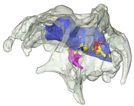
This Eocene Antarctic fossil penguin skull was discovered at La Meseta Formation at Seymour Island. Credit: Journal of Vertebrate Paleontology
When they’re not being the stars of various animated movies, penguins are playing an important role in evolutionary studies. Penguins are unique among modern birds in that they ‘fly’ through the water. Although flightless in air, penguins have a number of adaptations which allow them glide effortlessly through the water. And some of these adaptations are in an unlikely part of their anatomy — their brains. Recent finds of fossil penguins from 35 million year old sediments in Antarctica have begun to shed light on the changes in penguin brains that accompanied their transition to water.
“Comparing multiple species (extinct and living penguins and living birds that both fly and dive), in the way our study does, brings us closer to the answers of two major questions about penguin brain evolution: (1) what major morphological changes have occurred, (2) when did these changes occur?” said lead author Claudia Tambussi. The new finds, which are described in the latest issue of the Journal of Vertebrate Paleontology, include skulls which are so well-preserved that they could be CT-scanned to analyze their internal structure.
These scans revealed some interesting traits of these early penguins that speak to their transitional nature. Many of these findings have to do with the sensory abilities of these fossil species. For instance, one area, the Wulst, which is associated with complex visual functions, is enlarged. “The Antarctic fossils reveal that the neuroanatomy of penguins was still evolving roughly 30 million years after the loss of aerial flight, with trends such as the expansion of the Wulst and reduction of the olfactory bulbs still in progress,” said co-author Daniel Ksepka.
In addition to the increase in visual complexity, and reduction in olfaction, findings in the ear region shed light on the head position and equilibrium-maintaining abilities of the fossil penguins. All together, the findings show that these early penguins had many of the adaptations of living forms, while having a few unique traits not seen in the modern ones. Not only that, but some of these adaptations are found in modern flying birds, attesting to penguins’ unique mode of swimming.
Said Ksepka, “Penguins are considered flightless, but when it comes to wing-propelled diving they are essentially practicing underwater flight. The brain morphology reflects this as penguins retain an overall “flight-ready” brain.”
Video:
In this video, one of the Antarctic Eocene skulls is featured. The virtual brain is in blue: in red the right inner ear and carotids; in yellow the olfactory bulbs and some nerves.
Credit: Journal of Vertebrate Paleontology
Reference:
Claudia P. Tambussi, Federico J. Degrange, Daniel T. Ksepka. Endocranial anatomy of Antarctic Eocene stem penguins: implications for sensory system evolution in Sphenisciformes (Aves). Journal of Vertebrate Paleontology, 2015; e981635 DOI: 10.1080/02724634.2015.981635
The cave lion, Panthera leo spelaea. Credit: Encyclopedia Brittanica
ANSTO researchers using accelerator mass spectrometry (AMS) capabilities have assisted Russian palaeobiologists in dating rare fossils from an extinct cave lion that had been preserved in permafrost.
In collaborative research reported in the 17 August edition of Cosmos, research scientist Vladimir Levchenko and chemist Fiona Bertuch dated a fossilised bone, claw and hair found among the remnants of a near-complete skeleton of Panthera leo spelaea from a site in northeastern Russia.
Using ANSTO’s ultrasensitive dating techniques, Levchenko determined the age of the bone to be over 61,000 years. “Because this sample came from permafrost and was relatively well preserved, there was enough good quality collagen to work with,” said Levchenko.
Carbon extracted from animal hair was dated to 28,700 years but the inconsistency with the bone may be explained by contaminants in the fur.
Russian researchers led by I Kirillova of the Ice Age Museum in Moscow published their study in Quaternary Science Reviews following the discovery of 67 individual fossils in the Bilibino District of the Chukchi Autonomous Region in northeastern Russia.
The fossils were found submerged along a steep bank of the Malyi Anyui River. It is believed to be the first skeleton of a cave lion to be found in Russia. The cave lion got its name because of the large numbers of lion fossils found in caves. It lived at the same time as Neanderthals and has been depicted in cave art.
Investigators believe the cave lion was a healthy male, about 12 years old, whose diet largely consisted of bison and horses. Isotope measurements in Russia were used to confirm the prey consumed by the cave lion.
Reference:
“On the discovery of a cave lion from the Malyi Anyui River (Chukotka, Russia),” Quaternary Science Reviews, Volume 117, 1 June 2015, Pages 135-151, ISSN 0277-3791, DOI: 10.1016/j.quascirev.2015.03.029
ParaViewGeo is a free, BSD-licensed, open source visualization package for the exploration and mining industry.
ParaView is an open-source, multi-platform data analysis and visualization application. ParaView users can quickly build visualizations to analyze their data using qualitative and quantitative techniques. The data exploration can be done interactively in 3D or programmatically using ParaView’s batch processing capabilities.
ParaView was developed to analyze extremely large datasets using distributed memory computing resources. It can be run on supercomputers to analyze datasets of petascale size as well as on laptops for smaller data, has become an integral tool in many national laboratories, universities and industry, and has won several awards related to high performance computation.
Large Data Visualization Made Easier
ParaView is an open-source, multi-platform data analysis and visualization application. ParaView users can quickly build visualizations to analyze their data using qualitative and quantitative techniques. The data exploration can be done interactively in 3D or programmatically using ParaView’s batch processing capabilities. ParaView was developed to analyze extremely large datasets using distributed memory computing resources. It can be run on supercomputers to analyze datasets of petascale as well as on laptops for smaller data. ParaView is an application framework as well as a turn-key application.
The ParaView code base is designed in such a way that all of its components can be reused to quickly develop vertical applications. This flexibility allows ParaView developers to quickly develop applications that have specific functionality for a specific problem domain. ParaView runs on distributed and shared memory parallel and single processor systems. It has been successfully deployed on Windows, Mac OS X, Linux, SGI, IBM Blue Gene, Cray and various Unix workstations, clusters and supercomputers. Under the hood, ParaView uses the Visualization Toolkit (VTK) as the data processing and rendering engine and has a user interface written using Qt® The goals of the ParaView team include the following:
Develop an open-source, multi-platform visualization application.
Support distributed computation models to process large data sets.
Create an open, flexible, and intuitive user interface.
Develop an extensible architecture based on open standards.
The History of ParaView
The ParaView project started in 2000 as a collaborative effort between Kitware Inc. and Los Alamos National Laboratory. The initial funding was provided by a three-year contract with the US Department of Energy ASCI Views program. The first public release, ParaView 0.6, was announced in October 2002.
Independent of ParaView, Kitware started developing a web-based visualization system in December 2001. This project was funded by Phase I and II SBIRs from the US Army Research Laboratory and eventually became the ParaView Enterprise Edition. PVEE significantly contributed to the development of ParaView’s client/server architecture.
Since the beginning of the project, Kitware has successfully collaborated with Sandia, Los Alamos National Laboratories, the Army Research Laboratory and various other academic and government institutions to continue development. The project is still going strong!
In September 2005, Kitware, Sandia National Labs and CSimSoft started the development of ParaView 3.0. This was a major effort focused on rewriting the user interface to be more user-friendly and on developing a quantitative analysis framework. ParaView 3.0 was released in May 2007.
Use ParaViewGeo For
Research
We encourage the use of ParaViewGeo by students, professors and researchers alike. Being an open source program, it is free of charge and licensing fees. The program can also be customized and modified by users with programming experience—the source code is readily available. As more and more people use ParaViewGeo, we hope to have a community to offer feedback and support in the ongoing development of the software. For examples of how Kitware’s ParaView is used for scientific and academic purposes, visit ParaView’s Applications page.
Mining
The benefits of visualization extend beyond the exploration process. Mine design, planning and scheduling are all tasks that can be undertaken with ParaViewGeo. The process is made easier thanks to the wide range of different files (over 50 formats) that can be imported as source data for your model.
Over the past 10 years, MIRARCO has proven the value of visualization in mining. A number of large mining companies have undertaken strategic technical property reviews and effective investor relations presentations in a Virtual Reality Laboratory.ParaViewGeo is making this tool accessible to mining companies of all sizes for a number of different purposes throughout the mining process.
Geoscience
Geoscience is a broad and diverse field but the use of visualization is a commonality you’ll find in many of the sub-disciplines.ParaViewGeo has been used for geological, seismic and geomagnetic applications but the possibilities go far beyond these areas.ParaViewGeo can read a large number of file formats so that geological databases can be read and integrated into detailed spatial visualizations. This can be done with datasets big and small; ParaViewGeo can handle terabyte-size datasets.
MIRARCO’s Seismic Excavation Hazard Mapping System is a prime example of ParaViewGeo’s value to professional geoscientists. The system relies on ParaViewGeo to create detailed hazard maps for ground control personnel.
Exploration
Visualization has become a standard tool in the mining exploration trade and ParaViewGeo was developed specifically to meet the needs of exploration professionals.
ParaViewGeo reads over 50 different file formats and allows for the creation of integrated 3D models that can be manipulated and customized as the user sees fit. The software’s ability to handle terabyte-size datasets allows users to integrate all pertinent data for the most comprehensive property analysis and profitable decision making.
A sample dataset of the Brunswick Mine is included with every ParaViewGeo download.
Screenshot
Global Seismic Wave Propagation Simulation Contributors from ICES, The University of Texas at Austin: Carsten Burstedde, Omar Ghattas, James R. Martin, Georg Stadler, Lucas C. Wilcox Visualization at the Texas Advanced Computing Center, the University of Texas at Austin by Greg Abram
Golevka Asteroid Explosion Simulation. Image courtesy of Sandia Labs.Volcano-cone Acoustic-pressure Simulations ParaView was recently used in Russell Taylor’s Comp 715: Visualization in the Sciences class at the University of North Carolina at Chapel Hill. Author: Michael Garrett Larson and Alexander D. Hill Copyright: Data courtesy of Jonathan Lees and Keehoon Kim, UNC Geological Sciences
Damage in Montana is seen from the August 1959 Hebgen Lake earthquake. Credit: USGS
It’s not a huge mystery why Los Angeles experiences earthquakes. The city sits near a boundary between two tectonic plates — they shift, we shake. But what about places that aren’t along tectonic plate boundaries?
For example, seismicity on the North American plate occurs as far afield as southern Missouri, where earthquakes between 1811 and 1812 estimated at around magnitude 7 caused the Mississippi River to flow backward for hours.
Until now, the cause of that seismicity has remained unclear.
While earthquakes along tectonic plate boundaries are caused by motion between the plates, earthquakes away from fault lines are primarily driven by motion beneath the plates, according to a new study published by USC scientist Thorsten Becker in Nature on Aug. 27.
Just beneath the Earth’s crust is a layer of hot, semi-liquid rock that is continually flowing — heating up and rising, then cooling and sinking. That convective process, interacting with the ever-changing motion of the plates at the surface, is driving intraplate seismicity and determining in large part where those earthquakes occur. To a lesser extent, the structure of the crust above also influences the location, according to their models.
“This will not be the last word on the origin of strange earthquakes. However, our work shows how imaging advances in seismology can be combined with mantle flow modeling to probe the links between seismicity and mantle convection,” said Becker, lead author of the study and professor of Earth sciences at the USC Dornsife College of Letters, Arts and Sciences.
Becker and his team used an updated mantle flow model to study the motion beneath the mountain belt that cuts north to south through the interior of the Western United States.
The area is seismically active — the reason Yellowstone has geysers is that it sits atop a volcanic hotspot. Previously, scientists had suggested that the varying density of the plates was the main cause. (Imagine a mountain’s own weight causing it to want to flow apart and thin out.)
Instead, the team found that the small-scale convective currents beneath the plate correlated with seismic events above in a predictable way. They also tried using the varying plate density or “gravitational potential energy variations” to predict seismic events and found a much poorer correlation.
“This study shows a direct link between deep convection and shallow earthquakes that we didn’t anticipate, and it charts a course for improved seismic hazard mapping in plate interiors,” said Tony Lowry, co-author of the paper and associate professor of geophysics and geodynamics at Utah State University.
Reference:
Thorsten W. Becker, Anthony R. Lowry, Claudio Faccenna, Brandon Schmandt, Adrian Borsa, Chunquan Yu. Western US intermountain seismicity caused by changes in upper mantle flow. Nature, 2015; 524 (7566): 458 DOI: 10.1038/nature14867
A June 2015 map of the USArray component of the National Science Foundation-funded Earthscope project. Earthscope is a continental-scale seismic observatory designed to support integrated studies of continental lithosphere and deep Earth structure. Scientists from Utah State University, the University of Southern California, Roma Tre University, the University of New Mexico, Scripps and MIT used data collected from the project to study seismicity of the Intermountain Seismic Belt. They published findings in Nature. Credit: Earthscope.
Much of what we understand about earthquakes is based on plate tectonics. But for residents of Utah’s seismically restless Wasatch Front, a 120-mile-long metropolitan region anchored by Salt Lake City and bounded by the steep Wasatch Mountains and Great Salt Lake, such theory has fundamental limitations.
Because the state’s population center sits deep within the interior of the North American Plate, reasons why the Wasatch Fault is earthquake-prone, while other parts of the state are quieter, are poorly understood.
Plate motions across California’s San Andreas Fault, the Utah capitol’s nearest plate boundary some 760 miles away, don’t give a clear picture of what’s happening across the Beehive state and other areas of the Intermountain Seismic Belt, says Utah State University geophysicist Tony Lowry.
“In continental interiors, we know little about the forces that drive the earthquake cycle,” he says. “We rely mostly on the history of past earthquakes to assess hazards. But, because seismic observations cover only a tiny fraction of the time between the largest earthquakes, we can easily miss important parts of the story.”
Lowry suggests mantle flow stress, occurring deep within the earth, gives new insight into potential hazards that could shake the intraplate belt, which stretches from southwestern Utah up through Idaho and Wyoming to Yellowstone National Park and north through western Montana to Canada. He and colleagues Thorsten Becker of the University of Southern California, Claudio Faccenna of Italy’s Roma Tre University, Brandon Schmandt of The University of New Mexico, Adrian Borsa of the University of San Diego’s Scripps Institution of Oceanography and Chunquan Yu of the Massachusetts Institute of Technology publish the foundation of an emerging model in the August 27, 2015 issue of Nature. Their research is supported by the National Science Foundation.
“We’ve explored various aspects of how and why rocks break and flow, but this is the first time we’ve recognized the importance of deep mantle flow,” says Lowry, associate professor in USU’s Department of Geology. “This developing model gives us a new tool for understanding what makes earthquakes tick.”
In the past decade or so, researchers have focused on three possible mechanisms driving earthquakes. One is variations in gravitational potential energy, another is changes in thickness of the earth’s crust along the Intermountain Belt and the third is changes in strength of the lithosphere; that is, the crust and upper mantle.
Using new seismic and GPS data available from the massive NSF-funded Earthscope array across the western United States, the researchers looked at these observations simultaneously and found some surprises.
“In our earlier work, we tried to understand how deep mantle flow contributed to high elevations in the western United States,” Lowry says. “Thorsten (Becker) pushed us to explore whether or not elevation changes predicted by the same mantle flow models could explain the uplift we were observing with the Earthscope GPS measurements.”
It turns out the model did a poor job of explaining the GPS uplift, but gave a remarkable approximation of where to find earthquake belts because the upward push by mantle flow instead stretches the strong upper layer where earthquakes occur.
“Our findings represent the birth of a new idea and lay the groundwork for a better understanding of earthquakes,” Lowry says. “We now know we need to be looking for the impetus – that nudge that sets an earthquake system in motion – from flow at depths of 60 to 100 miles, much deeper than where we’d been looking.”
Becker, lead author on the paper, says the team’s work won’t be the last word on the origin of intraplate earthquakes.
“Our work shows how imaging advances in seismology can be combined with mantle flow modeling to probe the links between seismicity and mantle convection,” he says.
Reference:
Thorsten W. Becker, Anthony R. Lowry, Claudio Faccenna, Brandon Schmandt, Adrian Borsa& Chunquan Yu. Western US intermountain seismicity caused by changes in upper mantle flow. DOI:10.1038/nature14867
A fossilized Anchioris huxleyi, a bird-lke dinosaur, carries evidence of pigment and the subcellular organelles that made it. Credit: Thierry Hubin/RBINS
A study provides multiple lines of new evidence that pigments and the microbodies that produce them can remain evident in a dinosaur fossil. In the journal Scientific Reports, an international team of paleontologists correlates the distinct chemical signature of animal pigment with physical evidence of melanosome organelles in the fossilized feathers of Anchiornis huxleyi, a bird-like dinosaur that died about 150 million years ago in China.
The idea that melanosomes, which produce melanin pigment, are preserved in fossils has been hotly debated among scientists during the last several years. Microscopic traces that to some scientists seem to resemble melanosomes, appear to skeptics to instead be similar-looking bacteria. The new study resolves the debate, said co-author Ryan Carney, a graduate student at Brown University, by adding a powerful second line of evidence: chemistry.
“We have integrated structural and molecular evidence that demonstrates that melanosomes do persist in the fossil record,” said Carney, who helped design and write the study. “This evidence of animal-specific melanin in fossil feathers is the final nail in the coffin that shows that these microbodies are indeed melanosomes and not microbes.”
The finding has important implications for the interpretation of both past and future studies on fossil color, Carney said, and substantiates prior proposals that Anchiornis had some dark black feathers.
Signatures of animal pigment
In the new study, led by Johan Lindgren of Lund University in Sweden, the team used electron microscopes to observe what appear to be rod-like melanosome structures and imprints within the barbules of feathers all over the body.
That morphological evidence alone, however, would not advance the debate, so in addition the team performed two different kinds of chemical analyses to see if they could detect animal eumelanin pigment. They used both time-of-flight secondary ion mass spectrometry and infrared reflectance spectroscopy to discern the molecular signature of melanin in the samples. They compared those observed signatures with the signatures of modern-day animal eumelanin. The melanins were virtually identical, except for minor contributions from sulfur in the fossil, Carney said.
The researchers also analyzed the observed spectral signatures to compare them with melanins produced by various microbes, just to make sure that the pigments were not from any other source. The closest spectral agreement remained with an animal source, however.
“This is animal melanin, not microbial melanin, and it is associated with these melanosome-like structures in the fossil feathers,” Carney said.
Furthermore, no other types of molecules from potential microbes were detected.
Reference:
Johan Lindgren, Peter Sjövall, Ryan M. Carney, Aude Cincotta, Per Uvdal, Steven W. Hutcheson, Ola Gustafsson, Ulysse Lefèvre, François Escuillié, Jimmy Heimdal, Anders Engdahl, Johan A. Gren, Benjamin P. Kear, Kazumasa Wakamatsu, Johan Yans & Pascal Godefroit. Molecular composition and ultrastructure of Jurassic paravian feathers. Scientific Reports 5, Article number: 13520 (2015). DOI:10.1038/srep13520
The study looked at Thaumarchaeota archaea, which are found throughout the world’s oceans. These single-celled organisms have one membrane sac that encloses their bodies. This organism, used in the study, was collected from a tropical-water tank at the Seattle Aquarium. Credit: University of Washington
Understanding the planet’s history is crucial if we are to predict its future. While some records are preserved in ice cores or tree rings, other records of the climate’s ancient past are buried deep in the seafloor.
An increasingly popular method to deduce historic sea surface temperatures uses sediment-entombed bodies of marine archaea, one of Earth’s most ancient and resilient creatures, as a 150-million-year record of ocean temperatures. While other measures have gaps, this one is increasingly popular because it promises to fill in gaps to provide a near-global record of ocean temperatures going back to the age of the dinosaurs.
But University of Washington research shows this measure has a major hitch: The single-celled organism’s growth varies based on changes in ocean oxygen levels. Results published in August in the Proceedings of the National Academy of Sciences show that oxygen deprivation can alter the temperature calculations by as much as 21 degrees Celsius.
“It turned out that oxygen has a huge, dramatic effect,” said corresponding author Anitra Ingalls, a UW associate professor of oceanography. “It’s a big problem.”
Recent research shows these archaea, which draw energy from mere whiffs of ammonia, make up about 20 percent of microbial life in the oceans. Their bodies are plentiful in the ocean floor.
A method established in 2002 uses fats in the archaea’s cell membrane to measure past ocean temperatures, including during a major warming event about 56 million years ago that is one of the best historical analogs for present-day climate change, and a sudden oceanic cooling of up to 11 degrees Celsius during a period of low ocean oxygen about 100 million years ago, when other records are scarce.
Climate scientists found they could measure ocean temperature by looking at the change in the TEX-86 index, a temperature proxy named for the 86-carbon lipids in the cell membrane, which often tracks the surrounding water temperature.
The method seems to work better in some samples than others, prompting Ingalls and her co-authors to wonder about its physiological basis. The newly published experiments tested that relationship and found an unexpectedly strong response to low oxygen.
“Changing the oxygen gives us as much as 21 degree Celsius shift in the reading,” said first author Wei Qin, a UW doctoral student in civil and environmental engineering. “That’s solid evidence that it’s not just a temperature index.”
This means the TEX-86 measurements are inaccurate in parts of the ocean that may have experienced oxygen changes at the same time — for example, in low-oxygen zones or during major extinction events. This is exactly when the archaea are a popular index since other life forms, whose shells can provide a chemical signature for their growth temperatures, are absent.
It’s not known exactly why the archaea shift their lipid membranes. They may adapt to a temperature change by making their membrane tighter or less brittle in the new environment, Ingalls said. Low oxygen is another big environmental stressor.
“The envelope that encloses the cell is sort of the gatekeeper, and when stress is encountered of any kind, that membrane needs to adjust,” Ingalls said.
The new study is the first to actually look at how these archaea grow in different temperatures. These archaea are famously hardy — it’s the same group that lives in Yellowstone hot springs — but they have stymied attempts to grow them in captivity.
Qin was first author of a 2014 study that was the first to grow and compare individual strains of the marine Thaumarchaeota archaea under different conditions. He used samples from Puget Sound, a Seattle beach and a tropical-water tank at the Seattle Aquarium to show that related strains occupy a wide range of ecological niches.
In the new paper, he shows that the membrane lipids of different strains can have different temperature dependences. Some of them are a straight line, meaning they would be a good indication of past temperature, but others are not.
He also did experiments in which he changed the oxygen concentration of the air above the culture flasks. Results show that as the oxygen level drops, the TEX-86 measures rise dramatically, with reading spanning 15 to 36 degrees C even though all samples were grown at 26 C.
“This index provides an amazing historical record, but it’s very important how you understand it,” Qin said. “Otherwise it could be misleading.”
Knowing that oxygen affects the membrane structure can help improve interpretation of the TEX-86 record. Researchers can disregard samples from low-oxygen water to improve the accuracy of the technique, which as it is used now has error bars of about 2 degrees C.
“Plus or minus 2 degrees is not very good when you think about the sensitivity of the climate system,” Ingalls said. “This gives us a new way of thinking about the data.”
Next, the UW team hopes to do more experiments to learn how other factors, like nutrient levels and pH, affect these archaea’s metabolisms.
“We think there’s reason to believe that there’s all kinds of things that could affect the membrane lipid composition, not just temperature,” Ingalls said.
Reference:
Wei Qin, Laura T. Carlson, E. Virginia Armbrust, Allan H. Devol, James W. Moffett, David A. Stahl, Anitra E. Ingalls. Confounding effects of oxygen and temperature on the TEX86signature of marine Thaumarchaeota. Proceedings of the National Academy of Sciences, 2015; 201501568 DOI: 10.1073/pnas.1501568112
There’s gold in them thar volcanoes. Geoscientists have uncovered a mother lode of gold- and silver-enriched water in reservoirs inside a series of New Zealand volcanoes.
A shallow glob of magma heats water in the Taupo Volcanic Zone from below. The scalding water breaks down nearby rock and becomes loaded with dissolved metals such as gold and silver.
While subsurface rocks contain modest amounts of gold, researchers identified six water reservoirs hundreds of meters deep that brim with bling. Gold concentrations in the water topped 20 parts per billion and silver concentrations reached 2,000 or more parts per billion. Geoscientist Stuart Simmons of the University of Utah in Salt Lake City and colleagues report their findings in a paper to be published in Geothermics.
Tapping one of these water reservoirs could yield as much as $2.71 million of gold and $3.6 million of silver annually, the researchers estimate. Hopeful prospectors should note, however, that safe extraction may require the development of new mining technologies to avoid interfering with a way people are already tapping into the volcanoes’ riches: by converting their heat into electricity.
Malformed (a) versus normal (b) plankton. Toxic metal contamination may be a previously unrecognized contributing agent to many, if not all, extinction events in the ancient oceans. Credit: Image courtesy of Ghent University
Several Palaeozoic mass extinction events during the Ordovician and Silurian periods (ca. 485 to 420 to million years ago) shaped the evolution of life on our planet. Although some of these short-lived, periodic events were responsible for eradication of up to 85% of marine species, the exact kill-mechanism responsible for these crises remains poorly understood.
An international team led by Thijs Vandenbroucke (researcher at the French CNRS and invited professor at UGent) and Poul Emsbo (US Geological Survey) initiated a study to investigate a little known association between ‘teratological’ or ‘malformed’ fossil plankton assemblages coincident with the initial stages of these extinction events.
In a paper just published in Nature Communications, they present evidence that malformed fossil remains of marine plankton from the late Silurian (415 million years ago) contain highly elevated concentrations of heavy metals, such as iron, lead, and arsenic. These are well-known toxins that cause morphologic abnormalities in modern aquatic organisms; which led the authors to conclude that metal poisoning caused the malformation observed in these ancient organisms and may have contributed to their extinction and that of many other species.
Documented chemical behavior of these metals, which correlates with previously observed disturbances in oceanic carbon, oxygen and sulphur signatures, strongly suggests that these metal increases resulted from reductions of ocean oxygenation.
Thus, metal toxicity, and its expressions in fossilized malformations, could provide the ‘missing link’ that relates organism extinctions to widespread ocean anoxia. As part of a series of complex systemic interactions accompanying oceanic geochemical variation, the mobilisation of metals in spreading anoxic waters may identify the early phase of the kill-mechanism that culminated in these catastrophic events.
The recurring correlation between fossil malformations and Ordovician-Silurian extinction events raises the provocative prospect that toxic metal contamination may be a previously unrecognized contributing agent to many, if not all, extinction events in the ancient oceans.
Reference:
Thijs R. A. Vandenbroucke, Poul Emsbo, Axel Munnecke, Nicolas Nuns, Ludovic Duponchel, Kevin Lepot, Melesio Quijada, Florentin Paris, Thomas Servais, Wolfgang Kiessling. Metal-induced malformations in early Palaeozoic plankton are harbingers of mass extinction. Nature Communications, 2015; 6: 7966 DOI: 10.1038/ncomms8966
This is an illustration of Gueragama sulamerica. Credit: Julius Csotonyi
University of Alberta paleontologists have discovered a new species of lizard, named Gueragama sulamericana, in the municipality of Cruzeiro do Oeste in Southern Brazil in the rock outcrops of a Late Cretaceous desert, dated approximately 80 million years ago.
“The roughly 1700 species of iguanas are almost without exception restricted to the New World, primarily the Southern United States down to the tip of South America,” says Michael Caldwell, biological sciences professor from the University of Alberta and one of the study’s authors. Oddly however, iguanas closest relatives, including chameleons and bearded dragons, are all Old World. As one of the most diverse groups of extant lizards, spanning from acrodontan iguanians (meaning the teeth are fused to the top of their jaws) dominating the Old World to non-acrodontans in the New World, this new lizard species is the first acrodontan found in South America, suggesting both groups of ancient iguanians achieved a worldwide distribution before the final break up of Pangaea.
A terrestrial Noah’s Arc
“This fossil is an 80 million year old specimen of an acrodontan in the New World,” explains Caldwell. “It’s a missing link in the sense of the paleobiogeography and possibly the origins of the group, so it’s pretty good evidence to suggest that back in the lower part of the Cretaceous, the southern part of Pangaea was still a kind of single continental chunk.”
Distributions of plants and animals from the Late Cretaceous reflect the ancestry of Pangaea when it was whole. “This Gueragama sulamericana fossil indicates that the group is old, that it’s probably Southern Pangaean in its origin, and that after the break up, the acrodontans and chameleon group dominated in the Old World, and the iguanid side arose out of this acrodontan lineage that was left alone on South America,” says Caldwell. “South America remained isolated until about 5 million years ago. That’s when it bumps into North America, and we see this exchange of organism north and south. It was kind of like a floating Noah’s Arc for a very long time, about 100 million years. This is an Old World lizard in the new world at a time when we weren’t expecting to find it. It answers a few questions about iguanid lizards and their origin.”
The University of Alberta is a world leader in paleontology. This study was a collaboration between the University of Alberta and scientists in Brazil. Caldwell says of the collaboration, “It’s providing an opportunity for our students and research groups to expand our expertise and interests into an ever-increasing diversity of organisms within this group of animals called snakes and lizards.”
The lead author of the paper is Caldwell’s PhD student, Tiago Simoes, a Vanier scholar. “As with many other scientific findings, this one raises a number of questions we haven’t previously considered,” says Simoes. “This finding raises a number of biogeographic and faunal turnover questions of great interest to both paleontologists and herpetologists that we hope to answer in the future.”
In terms of next steps, Caldwell notes “Each answer only rattles the questions harder. The evolution of the group is much older than has been previously thought, which means we can push an acrodontan to 80 million years in South America. We now need to focus on much older units of of rock if we’re going to find the next step in the process.”
The findings, “A stem acrodontan lizard in the Cretaceous of Brazil revises early lizard evolution in Gondwana,” were published in the journal Nature Communications, one of the world’s top multidisciplinary scientific journals.
Reference:
Tiago R. Simões, Everton Wilner, Michael W. Caldwell, Luiz C. Weinschütz, Alexander W. A. Kellner. A stem acrodontan lizard in the Cretaceous of Brazil revises early lizard evolution in Gondwana. Nature Communications, 2015; 6: 8149 DOI: 10.1038/ncomms9149
Ice Age paleontologist Prof. Dr. Ralf-Dietrich Kahlke of the Senckenberg Research Station for Quaternary Paleontology in Weimar recorded the maximum geographic distribution of the woolly mammoth during the last Ice Age and published the most accurate global map in this regard. The ice-age pachyderms populated a total area of 33,301,000 square kilometers and may thus be called the most successful large mammals of this era. The study, recently published online in the scientific journal Quaternary International, determined that the distribution was limited by a number of climate-driven as well as climate-independent factors.
The mammoth is the quintessential symbol of the Ice Age — and the status of these shaggy pachyderms has now been confirmed scientifically. “The recent research findings show that during the last Ice Age, mammoths were the most widely distributed large mammals, thus rightfully serving as a flagship species of the glacial era,” according to Prof. Dr. Ralf-Dietrich Kahlke, an Ice Age researcher at the Senckenberg Research Station for Quaternary Paleontology in Weimar.
Kahlke has summarized the mammoth’s distribution during the most recent Ice Age, i.e., the period between approx. 110,000 and 12,000 years ago, on a worldwide map. All in all, the Weimar paleontologist determined a total distribution area of 33,301,000 square kilometers for these large mammals — almost 100 times the area of Germany today. From Portugal in the southwest across Central and Eastern Europe, Mongolia, Northern China, South Korea and Japan up to Northeastern Siberia, and thence to the American Midwest and Eastern Canada, from the shelf regions of the Arctic Ocean and Northwestern Europe to the bottom of the Adriatic Sea and to the mountains of Crimea: the fossil remains of woolly mammoths have been found everywhere.
“We related the computed distribution area to the real land surface at that time, thus generating the most precise map to date regarding the global habitats of the woolly mammoth,” explains Kahlke, and he adds, “Such detailed knowledge regarding the distribution area is not even available for many species of animals alive today.”
The generated map is based on decades of surveys of thousands of excavation sites on three continents. “Even sites under water, off the North American Atlantic shore and the North Sea, were taken into account. Due to the lower sea levels during the Ice Age — a large volume of water was bound in glaciers — these areas had fallen dry and were also inhabited by Mammuthus primigenius,” according to Kahlke.
Only the ice-age bison (Bison priscus) had a widespread distribution similar to that of the mammoths. Kahlke explains, “The bison were clearly more variable than the woolly mammoths. Obviously, the mammoths had a higher tolerance toward various environmental factors and they were able to successfully settle in a variety of rather different open landscapes.”
But there were certain factors that limited the distribution of the hirsute pachyderms: glaciers, mountain chains, semi-deserts and deserts, as well as changes in sea level and shifts in vegetation placed restrictions on the mammoths’ distribution area. “The analysis of these limiting factors is useful in understanding the distribution of fossil species and their extinction — as with the mammoths toward the end of the last Ice Age. In addition, the data aid in comprehending current changes in the distribution areas of recent animal species,” offers Kahlke in summary.
Reference:
Ralf-Dietrich Kahlke. The maximum geographic extension of Late Pleistocene Mammuthus primigenius (Proboscidea, Mammalia) and its limiting factors. Quaternary International, 2015; DOI: 10.1016/j.quaint.2015.03.023
These two Los Angeles area maps compare ground motions calculated by SCEC earthquake simulations to ground motions observed during the 2008 Chino Hills earthquake. On each map, the star marks the quake’s epicenter, and the dots show locations where ground motions were recorded for that earthquake. The color variations show how well the simulated ground motions match the observed ground motions, with darker colors (from red to black) indicating areas with poorer matches, and lighter colors (from yellow to white) indicating areas with good matches. The two maps show results from simulations using different 3-D Earth structure models. The Earth model that produced the best overall match to observations (here shown to the left) was the model used as input for the team’s recent 1 hertz CyberShake seismic hazard simulation on the Blue Waters supercomputer at the National Center for Supercomputing Applications (NCSA). Credit: Ricardo Taborda, University of Memphis, and Jacobo Bielak, Carnegie Mellon University
Earthquakes occur on a massive scale and often originate deep below the surface of the Earth, making them notoriously difficult to predict.
The Southern California Earthquake Center (SCEC) and its lead scientist, Thomas Jordan, use massive computing power made possible by the National Science Foundation (NSF) to improve our understanding of earthquakes. In doing so, SCEC is helping to provide long-term earthquake forecasts and more accurate hazard assessments.
One SCEC effort in particular, the PressOn project, aims to create more physically-realistic, wave-based earthquake simulations using an earthquake model they developed called CyberShake, which calculates how earthquake waves ripple through a 3-D model of the ground.
The latest NSF-funded supercomputers, capable of performing quadrillions of calculations every second, make this more accurate approach to studying earthquakes possible.
The Earth’s crust is made of plates that float on the molten outer core. Most earthquakes result from these plates moving relative to one another, a process called plate tectonics.
The edges of plates are rough. Those edges get stuck on one another while the rest of the plates keep moving, storing up energy—a process like stretching a rubber band. When the plate edges finally come unstuck (like letting go of one end of the rubber band), all the pent-up energy is released and the plate jerks into place. Aftershocks happen when the plate overshoots its equilibrium point and continues to readjust over the coming days to years.
Three distinct types of wave are generated by an earthquake: primary waves, secondary waves and surface waves. Each has a unique behavior and a distinct signature. The characteristics, timing and damage pattern of these waves differ by distance from the origin of the earthquake and the type of rock or soil they move through.
Given detailed information about the geological material in specific areas, physics-based 3-D wave propagation simulations are able to calculate how earthquake waves will move through the Earth and how strong the ground motions will be when the waves reach the surface.
In 2014, the SCEC team investigated the earthquake potential of the Los Angeles Basin, where the Pacific and North American plates run into each other at the San Andreas Fault. In this study, the simulation showed earthquake waves trapped, and reverberating, within in the Los Angeles basin. The high-shaking ground motions were much more than Jordan and his team expected.
“These basins act as essentially big bowls of jelly that shake during earthquakes and therefore very much affect the motion,” Jordan said.
SCEC’s simulations vary in terms of seismic wave cycles per second, or hertz. As that measurement increases, so does the potential for damage—and the complexity of the simulation. Structures such as buildings and bridges are most vulnerable to damage by seismic waves between 1 and 10 hertz.
The team first simulated individual earthquakes at 4 hertz. They then performed a simulation involving a large ensemble of earthquakes at 1 hertz—simulating more quakes required lowering the wave intensity—to calculate a probabilistic seismic hazard model for the Los Angeles area. A seismic hazard model describes the probability that an earthquake will occur in a given geographic area, within a given window of time, and with ground motion intensity exceeding a given threshold.
Starting in April 2015 and continuing over seven weeks, SCEC used the NSF-funded Blue Waters and Titan supercomputers at the Oak Ridge Leadership Computing Facility to calculate the first 1 hertz CyberShake hazard model specific to the Los Angeles Basin. This simulation doubled the maximum simulated frequency of the previous year’s CyberShake seismic hazard model, therefore also doubling the accuracy.
Even though the number of calculations required increased as the maximum simulated frequency of the earthquake went up, the tremendous computing power of Blue Waters and Titan reduced the time needed for these calculations from months to weeks.
Scientists believe seismic hazard analyses need to simulate earthquake frequencies above 10 hertz to realistically capture the full dynamics of a potential event. SCEC’s work is paving the way for those simulations. Physics-based 3-D earthquake simulations at 10 hertz, once a distant dream, are now on the horizon.
The mineral hazenite, named after Robert Hazen, which is only found in one locality, Mono Lake, Calif. Like hazenite, 22 percent of known minerals are found in just one locality. The image is courtesy of Courtesy of Hexiong Yang. Credit: Hexiong Yang
New research from a team led by Carnegie’s Robert Hazen predicts that Earth has more than 1,500 undiscovered minerals and that the exact mineral diversity of our planet is unique and could not be duplicated anywhere in the cosmos.
Minerals form from novel combinations of elements. These combinations can be facilitated by both geological activity, including volcanoes, plate tectonics, and water-rock interactions, and biological activity, such as chemical reactions with oxygen and organic material.
Nearly a decade ago, Hazen developed the idea that the diversity explosion of planet’s minerals from the dozen present at the birth of our Solar System to the nearly 5,000 types existing today arose primarily from the rise of life. More than two-thirds of known minerals can be linked directly or indirectly to biological activity, according to Hazen. Much of this is due to the rise of bacterial photosynthesis, which dramatically increased the atmospheric oxygen concentration about 2.4 billion years ago.
In a suite of four related, recently published papers, Hazen and his team–Ed Grew, Bob Downs, Joshua Golden, Grethe Hystad, and Alex Pires–took the mineral evolution concept one step further. They used both statistical models of ecosystem research and extensive analysis of mineralogical databases to explore questions of probability involving mineral distribution.
They discovered that the probability that a mineral “species” (defined by its unique combination of chemical composition and crystal structure) exists at only one locality is about 22 percent, whereas the probability that it is found at 10 or fewer locations is about 65 percent. Most mineral species are quite rare, in fact, found in 5 or fewer localities.
“Minerals follow the same kind of frequency of distribution as words in a book,” Hazen explained. “For example, the most-used words in a book are extremely common such as ‘and,’ ‘the,’ and ‘a.’ Rare words define the diversity of a book’s vocabulary. The same is true for minerals on Earth. Rare minerals define our planet’s mineralogical diversity.”
Further statistical analysis of mineral distribution and diversity suggested thousands of plausible rare minerals either still await discovery or occurred at some point in Earth’s history, only to be subsequently lost by burial, erosion, or subduction back into the mantle. The team predicted that 1,563 minerals exist on Earth today, but have yet to be discovered and described.
The distribution of these “missing” minerals is not uniform, however.
Several circumstances influence the likelihood of a mineral having previously been discovered. This includes physical characteristics, such as color. White minerals are less likely to have been noticed, for example. Other factors include the quality of crystallization, solubility in water, and stability near the surface of the planet.
As such, Hazen and his colleagues predicted that nearly 35 percent of sodium minerals remain undiscovered, because more than half of them are white, poorly crystallized, or water soluble. By contrast, fewer than 20 percent of copper, magnesium, and copper minerals have not been discovered.
Further expanding the link between geological and biological evolution, Hazen’s team applied the biological concepts of chance and necessity to mineral evolution. In biology, this idea means that natural selection occurs because of a random “chance” mutation in the genetic material of a living organism that becomes, if it confers reproductive advantage, a “necessary” adaptation.
But in this instance, Hazen’s team asked how the diversity and distribution of Earth’s minerals came into existence and the likelihood that it could be replicated elsewhere. What they found is that if we could turn back the clock and “re-play” Earth’s history, it is probable that many of the minerals formed and discovered in this alternate version of our planet would be different from those we know today.
“This means that despite the physical, chemical, and biological factors that control most of our planet’s mineral diversity, Earth’s mineralogy is unique in the cosmos,” Hazen said.
The four papers are published in Canadian Mineralogist, Mathematical Geoscience, American Mineralogist, and Earth and Planetary Science Letters.
The Ekati diamond mine, on the tundra of Canada’s Northwest Territories, source of some of Weiss’s samples. The geochemist is interested in the origins of North American diamonds.
Geochemist Yaakov Weiss deals in diamonds. Not the brilliant jewelry-store kind, but the flawed, dirty-looking ones used more for industry than decoration. Gem-grade diamonds are generally pure crystallized carbon, but many lower-grade stones contain so-called inclusions–chemical intruders bottled up inside the crystal. Inclusions lower the stone’s value; but they contain worlds of information about the deep, inaccessible regions where diamonds come from. Their compositions speak to not only how diamonds form (and maybe how to find them), but other basic processes below.
“They are the most pristine samples we can get from underlying depths,” says Weiss, who works at Columbia University’s Lamont-Doherty Earth Observatory. “After a diamond captures something, from that moment until millions of years later in my lab, that material stays the same. We can look at diamonds as time capsules, as messengers from a place we have no other way of seeing.” Some of his recent studies are providing new insights to these regions.
For most of history, almost everything about diamonds was a mystery; no one even knew where they came from. In the late 19th century, geologists figured out that they erupt in small, oddball volcanic spouts, called kimberlites. These eruptions usually punch through the centers of ancient continents, made of rocks that date back billions of years. The diamonds themselves may or may not be that old. Scientists now believe they crystallize in earth’s mantle, 140 to 250 kilometers (about 90 to 150 miles) below. A few may come from as deep as 700 kilometers (430 miles)–the deepest direct samples we have from those depths. At the surface, kimberlites are tiny–usually just a few acres–and hard to find. They are also mostly barren of diamonds; of around 1,500 or 2,000 known, only 50 or 60 have ever been found that are worth mining. Because diamonds are so valuable, many scientists are working to better understand them. But many questions remain. Exactly what raw materials and processes go into making diamonds? What causes kimberlites to erupt? Why are kimberlites, and diamonds, found in some areas, and not in others?
Weiss’s latest study, on the cover of the leading journal Nature, gets at some of these questions. In it, he and colleagues studied diamonds from the tundra of Canada’s Northwest Territories. Prospectors have hunted diamonds across the United States and Canada for centuries, but it was not until the 1990s that the continent’s first viable mines were discovered here. Some of the surface rocks are billions of years old, but the kimberlites that penetrated them are the youngest known–as young as 45 million years (others elsewhere can be hundreds of millions).
Working with colleagues from the University of Alberta and Durham University, Weiss investigated so called fibrous diamonds–inferior stones that consist of multiple layers instead of a single gem-grade crystal–from the rich Ekati Mine. Inside, they found tiny droplets of liquid–apparent remainders of raw material from which the diamonds crystallized. Most researchers believe that diamonds solidify out of some kind of fluid or fluids; but exactly what those fluids are, and what processes are involved, are controversial.
Analyses of these inclusions, and separate research on stones from a neighboring mine, showed them to be rich in carbon, and highly saline–plenty of chlorine, potassium and sodium, much like seawater. Weiss thinks this is not a coincidence. In recent years, other researchers have shown that the complex evolutions of the far north has included repeated opening and closing of ocean basins. A few have wondered if these events could be related to the formation of diamond-bearing kimberlites. Weiss and his colleagues connected the dots. Their research suggests that a slab of watery oceanic crust subducted at a shallow angle under the far more ancient continental rocks 150 million to 200 million years ago. The slab, they say, could have slid more or less intact, underneath what is now the present-day Canadian tundra, where the mines are located. There, they say, fluids from the long-traveled ocean crust reacted with solid continental rocks just above them, in exactly the zone where pressure and temperature conditions are right for forming diamonds. To bolster the case, in addition to the salts in the inclusions, there are trace element and isotope fingerprints that match the composition of seawater from this time, they say. Whether the reactions had something to do with driving the kimberlite eruptions to the surface is an open question.
Among other things, the study may help open the way to reconsidering the source of carbon for diamonds. As far as anyone can tell so far, most of the carbon seems to come from the depths of the mantle. But in recent years evidence has been building that at least some of it was once on the surface, and was shoved down by subducting tectonic plates like the ones Weiss proposes. A recent study by Lamont geochemist Peter Kelemen argues that the carbon can come from either the surface or the deep earth, though very little from either source gets turned into diamond. Weiss’s current study does not examine this question.
Are there more deposits to be found? Since the 1800s, scattered single diamonds have been found in many U.S. states and Canadian provinces, but almost none can be traced back to kimberlite sources. Some kimberlites have been uncovered, but most don’t contain diamonds. One small mine operated in rural Arkansas in the early 1900s was quickly worked out; it is now a state park, where amateur diggers occasionally still find diamonds. Diamondiferous kimberlite was found in Colorado in the 1970s, but it was too poor for mining. The processes described in the Northwest Territories might have taken place elsewhere, but that remains to be seen. “Now it’s time to look at fluid inclusions from other places,” says Weiss. “Maybe the same things are happening in other areas. Maybe not.”
Weiss continues to work on related questions. At any one time, he has about 100 diamonds used for research. They are generally fingernail-clipping-size chips from larger stones. He keeps them wrapped up in elaborately folded small papers, labeled with origin and other information. In addition to Canadian diamonds, he has stones from Zimbabwe, Guinea, South Africa, Siberia and Brazil. Most have been loans or gifts from friends or colleagues, though a few years back he paid about $700 to a dealer in his native Israel for a half-dozen 1.5-carat African stones.
Most of his investigations do not harm the diamonds; inclusions often can be analyzed by passing microscopic light beams or X-rays through them. However, in one new project aimed at diamonds from unusually deep regions, Weiss plans some destruction. To analyze isotopes of helium gas trapped within, he has to pulverize the diamonds to release the gas. (Diamond is the world’s hardest substance, almost impossible to wear down–but a direct whack with a hammer will shatter one. Repeated beating turns it to something resembling fine granulated sugar.) “It seems crazy to crush diamonds, right?” he admits. “But it’s the only way to get at that particular question.”
Last year, Weiss published another paper about tiny droplets of fluid found encased within African gem-grade diamonds. Such droplets are fairly common in boart diamonds–inferior specimens like the fibrous type–but not in gems. Many scientists contend that boart and gem-grade stones crystallize out of two different kinds of fluids. To test the idea, Weiss obtained two very rare single-crystal stones containing fluids–one from South Africa’s Finsch diamond mine, and one from a river deposit in Kankan, Guinea. The gems’ fluids turned out to be similar to those in boart–a challenge to conventional theory.
Such research could have practical applications. For one, greater knowledge of trace elements in diamond inclusions could lead to chemical “fingerprints” that would tell where commercial gems originated. This would allow better enforcement of the Kimberley Process, the 2003 UN agreement to blacklist so-called “blood diamonds” from nations where mining is controlled by warlords or corrupt governments. The process currently depends on paperwork that can be easily faked.
Beyond this, “understanding diamond formation can tell us about the deep earth’s carbon cycle, which we have very little knowledge about,” says Weiss. This is the long-term movement of vast amounts of carbon from the atmosphere and surface down into earth’s interior, via biological processes, chemical weathering, subduction of tectonic plates, and then back up again via large, more conventional volcanic eruptions. The cycle is thought to play key roles in controlling climate and biological evolution, and in unseen processes far below the surface.
For all his expertise, Weiss has to admit: he has yet to visit a diamond mine. As a student in Israel, he considered collecting samples in conflict-ridden areas of west Africa, but his adviser discouraged him. “He wanted me to stay in the lab and stay alive–not get killed in the field,” he says. The mines in northern Canada are safe, but hard to get to–far out on roadless tundra, accessible only by charter aircraft. “I’m still hoping, some day,” he says. “Diamonds–they’re a very nice stone. It would be fun some day to see where people are finding them.”
Reference:
“Highly saline fluids from a subducting slab as the source for fluid-rich diamonds.” Nature 524, 339–342 (20 August 2015) DOI: 10.1038/nature14857
“High-density fluids and the growth of monocrystalline diamonds,” Geochimica et Cosmochimica Acta, Volume 141, 15 September 2014, Pages 145-159, ISSN 0016-7037, DOI: 10.1016/j.gca.2014.05.050
The devastating 2004 Indian Ocean earthquake and tsunami that killed 230,000 people has raised questions among coastal residents about when the next big tsunami will strike. It’s a question that University of Rhode Island geologist Simon Engelhart knows cannot be answered with any precision.
But he and colleagues from Humboldt State University, Rutgers University and the Earth Observatory of Singapore, in collaboration with geologists from Indonesia, examined the geological record in northern Sumatra to better understand how frequently large earthquakes and tsunamis occur there. The research was published in the August edition of the journal Geology.
What they found was evidence that five to seven major tsunamis had occurred between 7,400 and 3,800 years ago, with an additional four to six tsunamis since that time. “We can surmise from this that a major earthquake and tsunami occurred about every 600 to 900 years,” said Engelhart, URI assistant professor of geosciences. “But those are maximum recurrences. We’re not at a point where we can predict earthquakes.”
The researchers examined a dozen sediment cores up to 6 meters long from two sites near the shoreline of Sumatra’s Aceh province. Within the sediments in the cores were three layers of soil containing mangrove pollen that dropped into the intertidal zone during earthquakes and were buried by tidal flat sediments. Sands above the soils contained species of marine organisms called foraminifera that live far offshore, evidence that the sand was brought onshore by ancient tsunamis.
Radiocarbon dating of these soil layers and associated sands found that local earthquakes causing tsunamis occurred about 7,000, 5,800 and 3,800 years ago. Two turbid layers in the cores containing more oceanic foraminifera were evidence of additional tsunamis that took place during the same period.
“The archive of sedimentary evidence in the cores doesn’t tell the whole story, though,” Engelhart said. “We had to figure out what the sea level was doing for the last 8,000 years to identify when we would find geological records of earthquakes and tsunamis.”
According to Engelhart, sea level rose rapidly in the Indian Ocean up until about 8,000 years ago, when it slowed to a rate that allowed sediment to accumulate in predictable layers, enabling present-day scientists to study the environment of the time. About 3,800 years ago, however, sea level gradually stopped rising and sediments no longer accumulated. Instead, wave action mixed up the newer sands, blurring the historic chronology.
Even so, the research team was able to calculate the proportion of sediment that came from offshore in tsunamis by examining the number of fossilized forams that are typically found far out at sea. From this, they concluded that four to six tsunamis struck Sumatra in the last 3,800 years.
For Engelhart, part of the relevance of this study is in the realization of the importance of sea level in conducting this type of analysis.
“You need to understand how sea level varied at a site before you can think about the methods to improve our understanding of how often earthquakes and tsunamis occur and how big they are,” he said. “The relative sea-level history of this region demonstrates that we couldn’t use the classic sedimentary methods to reconstruct earthquakes and tsunamis during the last 3,800 years at these sites.”
Understanding the relative sea-level history will be especially important when scientists conduct analyses of earthquake-prone areas like Alaska, Chile, Peru, Japan and New Zealand, all of which have sea level records that raise similar issues. Engelhart is already applying these findings to related studies in Alaska and the west coast of North America at Cascadia.