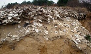
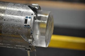
A typical Native American oyster deposit, or midden, dating to about 1,000 years ago. Credit: Torben Rick
Oysters are keystone organisms in estuaries around the world, influencing water quality, constructing habitat and providing food for humans and wildlife. Yet their populations in the Chesapeake Bay and elsewhere have dramatically declined after more than a century of overfishing, pollution, disease and habitat degradation. Smithsonian scientists and colleagues, however, have conducted the first bay-wide, millennial-scale study of oyster harvesting in the Chesapeake, revealing a sustainable model for future oyster restoration. Their research is published in the May 23 issue of the Proceedings of the National Academy of Sciences.
Despite providing food for humans for millennia, little is known about Chesapeake Bay oyster populations prior to the late 1800s. Using fossil, archaeological and modern biological data, the team of scientists was able to reconstruct changes in oyster size from four time frames: the Pleistocene (780,000-13,000 years ago), prehistoric Native American occupation (3,200-400 years ago), historic (400-50 years ago) and modern times (2000 to 2014).
They found that while oyster size fluctuated at certain points through time, it has generally decreased over time and the average size of modern oysters is significantly smaller than oysters from the 1800s and earlier.
“Our work demonstrates the importance of working across disciplines and using the past to help us understand and transcend modern environmental issues,” said Torben Rick, an anthropologist at the Smithsonian’s National Museum of Natural History and lead author of the research. “In this case, paleontology, archaeology, history and marine ecology all provided unique perspectives on the difficult puzzle of restoring Chesapeake oysters. Ultimately, they issue a challenge for us to make important and difficult decisions about how to restore and sustain our marine ecosystems and organisms.”
The team also found that Native Americans’ method of selecting and hand-collecting oysters likely resulted in more consistent average sizes and fewer very small individual oysters. People were likely removing oysters from the reefs in a way that was biased toward medium-sized oysters without decreasing the average size of the oysters in the harvested populations.
With limited variability in oyster size and abundance, and no strong evidence for a size decline from 3,500 to 400 years ago, the Native American Chesapeake Bay oyster harvesting appears to have been largely sustainable, despite changing climatic conditions and sea-level rise. The teams point to four supporting factors:
Water depth and technology restricted Native Americans’ harvest primarily close to shore
Oysters may have been harvested intensively at particular times of year and less so at others
The density of the human population was drastically lower than today
Broad-spectrum human diets that had a mix of marine and terrestrial resources
It is this sustainability of the Native American oyster fishery that can provide insight into the future restoration of oysters in the Chesapeake Bay and around the world. However, there are factors stacked against modern-day oysters that did not exist in the prehistoric Native American’s time.
“Chesapeake Bay oysters now face challenges resulting from disease, poor water quality and over a century of overfishing, which not only removes oysters, but also destroys the reef habitat oysters depend on,” said Denise Breitburg, co-author and senior scientist at the Smithsonian Environmental Research Center. “These factors have led to the decline of oysters in Chesapeake Bay and are making restoration difficult. But large-scale efforts are underway to try to reverse the trend.”
The team’s model of a sustainable prehistoric Native American harvest of oysters, primarily by hand from fringing reefs that left deeper-water reefs largely intact, supports recent plans for Chesapeake Bay oyster-restoration efforts. They include reduction of modern harvest levels and creation of increased no-take zones that are conceptually similar to deep-water areas where harvest was unlikely in Native American fisheries. Current restoration plans also include enhancement of oyster density using hatchery seed and the addition of new hard substrate where needed. The team’s Pleistocene data also provide a baseline against which the size distribution of oysters in no-take reserves could be evaluated.
While not solving all the challenges facing oysters in the Chesapeake, the team’s research provides an example of an apparently sustainable millennial-scale fishery, elements of which may help inform restoration and harvest in today’s ecosystem.
The archaeological component of this study was funded by the Smithsonian Institution and a Committee for Research and Exploration grant from the National Geographic Society.
Reference:
Millennial-scale sustainability of the Chesapeake Bay Native American oyster fishery, PNAS, DOI: 10.1073/pnas.1600019113
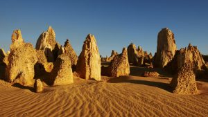
It’s a true desert landscape in Nambung National Park, where the weathered rock spires of the Pinnacles rise out of yellow sand dunes. Yet the park sits on the deep blue Indian Ocean, along an idyllic stretch of coast three hour’s drive north of Perth. After experiencing the eerie Pinnacles, stay in the fishing village of Cervantes, with its white beaches, coral reefs and Lake Thetis, a salt lake teeming with living fossils. Get up close to a rich array of wildlife in Badgingarra National Parks and discover Jurien Bay’s national parks and idyllic sandy beaches.
Formation
The raw material for the limestone of the Pinnacles came from seashells in an earlier era that was rich in marine life. These shells were broken down into lime-rich sands that were blown inland to form high mobile dunes. However, the manner in which such raw materials formed the Pinnacles is the subject of debate and three theories have been proposed.
The first theory states that they were formed as dissolutional remnants of the Tamala Limestone, i.e. that they formed as a result of a period of extensive solutional weathering (karstification). Focused solution initially formed small solutional depressions, mainly solution pipes, which were progressively enlarged over time, resulting in the pinnacle topography. Some pinnacles represent cemented void infills (microbialites and/or re-deposited sand), which are more resistant to erosion, but dissolution still played the final role in pinnacle development.
A second theory states that they were formed through the preservation of tree casts buried in coastal aeolianites, where roots became groundwater conduits, resulting in the precipitation of indurated (hard) calcrete. Subsequent wind erosion of the aeolianite then exposed the calcrete pillars.
A third proposal suggests that plants played an active role in the creation of the Pinnacles, based on the mechanism that formed smaller “root casts” in other parts of the world. As transpiration drew water through the soil to the roots, nutrients and other dissolved minerals flowed toward the root—a process termed “mass-flow” that can result in the accumulation of nutrients at the surface of the root, if the nutrients arrive in quantities greater than that needed for plant growth. In coastal aeolian sands that consist of large amounts of calcium (derived from marine shells), the movement of water to the roots would drive the flow of calcium to the root surface. This calcium accumulates at high concentrations around the roots and over time is converted into a calcrete. When the roots die, the space occupied by the root is subsequently also filled with a carbonate material derived from the calcium in the former tissue of the roots, and possibly also from water leaching through the structures. Although evidence has been provided for this mechanism in the formation of root casts in South Africa, evidence is still required for its role in the formation of the Pinnacles.
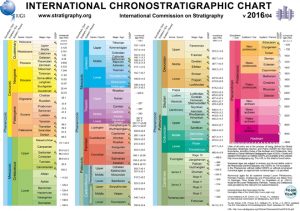
Click here (PDF or JPG) to download the latest version (v2016/04) of the International Chronostratigraphic Chart.
Translations of the chart: Chinese (v2015/01: PDF or JPG), Spanish (v2015/01: PDF or JPG), Basque (v2015/01: PDF or JPG), Catalan (v2015/01: PDF or JPG), Norwegian (v2015/01: PDF or JPG), Lithuanian (v2015/01: PDF or JPG), Japanese (v2014/02: PDF or JPG), Portuguese (v2013/01: PDF or JPG) and French (v2012).
The old versions can be download at the following links: 2008 (PDF or JPG), 2009 (PDF or JPG), 2010 (PDF or JPG), 2012 (PDF or JPG), 2013/01 (PDF or JPG), 2014/02 (PDF or JPG) , 2014/10 (PDF or JPG), 2015/01 (PDF or JPG) and the ChangeLog for 2012-2016.
Two hundred and fifty million years ago, life on earth was in a tail-spin—climate change, volcanic eruptions, and rising sea levels contributed to a mass extinction that makes the death of the dinosaurs look like child’s play. Marine life got hit hardest—96% of all marine species went extinct. For a long time, scientists believed that the early marine reptiles that came about after the mass extinction evolved slowly, but the recent discovery of a strange new fossil brings that view into question.
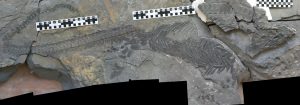
In a paper published in Scientific Reports, paleontologists describe a new marine reptile, Sclerocormus parviceps, an ichthyosauriform that’s breaking all the rules about what ichthyosaurs are like.
Ichthyosaurs were a massive group of marine reptiles that lived around the time of the earliest dinosaurs. Most of them looked a little bit like today’s dolphins—streamlined bodies, long beak-like snouts, and powerful tail fins. But the new species is something of a black sheep. It has a short snout (its species name even means “small skull”), and instead of a tail with triangular flukes (think of a fish’s tail-fins), it had a long, whip-like tail without big fins at the end. And while many ichthyosaurs had conical teeth for catching prey, Sclerocormus was toothless and instead seems to have used its short snout to create pressure and suck up food like a syringe. In short, it’s really different from most of its relatives, and that tells scientists something important about evolution.
“Sclerocormus tells us that ichthyosauriforms evolved and diversified rapidly at the end of the Lower Triassic period,” explains Olivier Rieppel, The Field Museum’s Rowe Family Curator of Evolutionary Biology. “We don’t have many marine reptile fossils from this period, so this specimen is important because it suggests that there’s diversity that hasn’t been uncovered yet.”
The way this new species evolved into such a different form so quickly sheds light on how evolution actually works. “Darwin’s model of evolution consists of small, gradual changes over a long period of time, and that’s not quite what we’re seeing here. These ichthyosauriforms seem to have evolved very quickly, in short bursts of lots of change, in leaps and bounds,” says Rieppel.
Animals like Sclerocormus that lived just after a mass extinction also reveal how life responds to huge environmental pressures. “We’re in a mass extinction right now, not one caused by volcanoes or meteorites, but by humans,” explains Rieppel. “So while the extinction 250 million years ago won’t tell us how to solve what’s going on today, it does bear on the evolutionary theory at work. How do we understand the recovery and rebuilding of a food chain, of an ecosystem? How does that get fixed, and what comes first?”
Note: The above post is reprinted from materials provided by Field Museum.
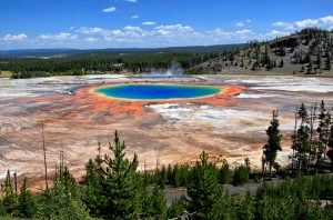
Grand Prismatic Spring in Yellowstone; such hot pools often bubble with undiscovered microbes. Credit: NPS
Earth could contain nearly 1 trillion species, with only one-thousandth of 1 percent now identified, according to the results of a new study.
The estimate, based on universal scaling laws applied to large datasets, appears today in the journal Proceedings of the National Academy of Sciences. The report’s authors are Jay Lennon and Kenneth Locey of Indiana University in Bloomington, Indiana.
The scientists combined microbial, plant and animal datasets from government, academic and citizen science sources, resulting in the largest compilation of its kind.
Altogether, these data represent more than 5.6 million microscopic and non-microscopic species from 35,000 locations across all the world’s oceans and continents, except Antarctica.
Great challenge in biology
“Estimating the number of species on Earth is among the great challenges in biology,” Lennon said. “Our study combines the largest available datasets with ecological models and new ecological rules for how biodiversity relates to abundance. This gave us a new and rigorous estimate for the number of microbial species on Earth.”
He added that “until recently, we’ve lacked the tools to truly estimate the number of microbial species in the natural environment. The advent of new genetic sequencing technology provides a large pool of new information.”
The work is funded by the National Science Foundation (NSF) Dimensions of Biodiversity program, an effort to transform our understanding of the scope of life on Earth by filling major gaps in knowledge of the planet’s biodiversity.
“This research offers a view of the extensive diversity of microbes on Earth,” said Simon Malcomber, director of the Dimensions of Biodiversity program. “It also highlights how much of that diversity still remains to be discovered and described.”
Estimating numbers of microbial species
Microbial species are forms of life too small to be seen with the naked eye, including single-celled organisms such as bacteria and archaea, as well as certain fungi.
Many earlier attempts to estimate the number of species on Earth ignored microorganisms or were informed by older datasets based on biased techniques or questionable extrapolations, Lennon said.
“Older estimates were based on efforts that dramatically under-sampled the diversity of microorganisms,” he added. “Before high-throughput genetic sequencing, scientists characterized diversity based on 100 individuals, when we know that a gram of soil contains up to a billion organisms, and the total number on Earth is more than 20 orders of magnitude greater.”
The realization that microorganisms were significantly under-sampled caused an explosion in new microbial sampling efforts over the past several years.
Extensive sampling efforts
The study’s inventory of data sources includes 20,376 sampling efforts on bacteria, archaea and microscopic fungi, as well as 14,862 sampling efforts on communities of trees, birds and mammals.
“A massive amount of data has been collected from these surveys,” said Locey. “Yet few have tried to pull together all the data to test big questions.”
He added that the scientists “suspected that aspects of biodiversity, like the number of species on Earth, would scale with the abundance of individual organisms. After analyzing a massive amount of data, we observed simple but powerful trends in how biodiversity changes across scales of abundance.”
Scaling laws for all species
The researchers found that the abundance of the most dominant species scales with the total number of individuals across 30 orders of magnitude, “making it the most expansive scaling law in biology,” says Lennon.
Scaling laws, like that discovered by the scientists, are known to accurately predict species numbers for plant and animal communities. For example, the number of species scales with the area of a landscape.
“Until now, we haven’t known whether aspects of biodiversity scale with something as simple as the abundance of organisms,” Locey said. “As it turns out, the relationships are not only simple but powerful, resulting in our estimate of upward of one trillion species.”
The study’s results also suggest that identifying every microbial species on Earth presents a huge challenge.
“Of those species cataloged, only about 10,000 have ever been grown in a lab, and fewer than 100,000 have classified genetic sequences,” Lennon said. “Our results show that this leaves 100,000 times more microorganisms awaiting discovery—and 100 million to be fully explored.
“Microbial biodiversity, it appears, is greater than we ever imagined.”
Reference:
Kenneth J. Locey et al. Scaling laws predict global microbial diversity, Proceedings of the National Academy of Sciences (2016). DOI: 10.1073/pnas.1521291113
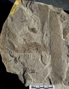
Macroscopic fossils preserved as carbonaceous compressions from the Gaoyuzhuang Formation (Mesoproterozoic Era) Credit: ZHU Maoyan
A research group led by Prof. ZHU Maoyan from Nanjing Institute of Geology and Paleontology reported on May 18 in Nature Communications the discovery of macroscopic fossils from the 1,560- million years (Myr)-old Gaoyuzhuang Formation, Yanshan area, North China, that exhibit both large size and regular morphology.
Preserved as carbonaceous compressions, the Gaoyuzhuang fossils have statistically regular linear to lanceolate shapes up to 30 cm long and nearly 8 cm wide, suggesting that the Gaoyuzhuang fossils record benthic multicellular eukaryotes of unprecedentedly large size. The new fossils provide the strongest evidence yet that multicellular eukaryotes with decimetric dimensions and a regular developmental program populated the marine biosphere at least a billion years before the Cambrian Explosion.
The fossils’ morphotypes are linear (elongate with parallel sides, truncated at both ends), cuneate (distinct taper on one end; other end truncated), oblong (rounded on one end) or tongue-shaped (round end, but without parallel sides) and so on. The tongue-shaped fossils are the largest remains in the assemblage, with dimensions up to 28.6 cm by 7.6 cm. The linear fossils are up 22.9 cm long and 4.5 cm wide with ragged ends, suggesting they are fragments of larger individuals.
The linear specimens resemble the distal ends of cuneate compressions, and size frequency distributions for the two morphotypes overlap strongly. The inference of organized multicellularity is reinforced by well-preserved cell sheets in organic fragments extracted from fossiliferous samples by acid maceration.
The Gaoyuzhuang fossils provide the most compelling evidence yet reported that by the beginning of the Mesoproterozoic Era, 1,600 Myr ago, eukaryotic organisms had evolved macroscopic form, multicellularity with limited cell differentiation, and (probably) photosynthesis. If so, their rarity as fossils in pre-Ediacaran (>635 Myr) must reflect processes of preservation rather than simple biological absence. Continuing research promises new insights into marine ecosystems in the low oxygen world caricatured misleadingly as a ‘boring billion’ year interval of evolutionary as well as environmental stability.
This study was supported by the National Natural Science Foundation of China and National Key Basic Research Program of China.
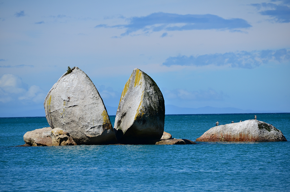
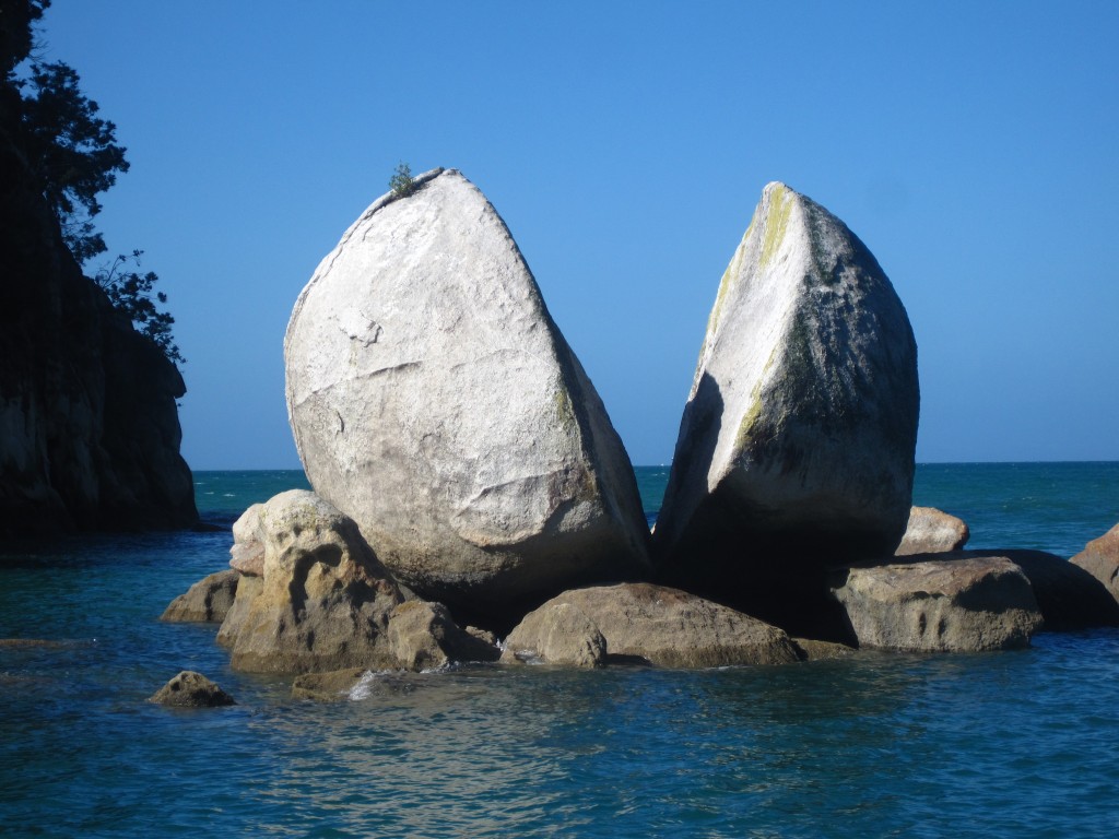
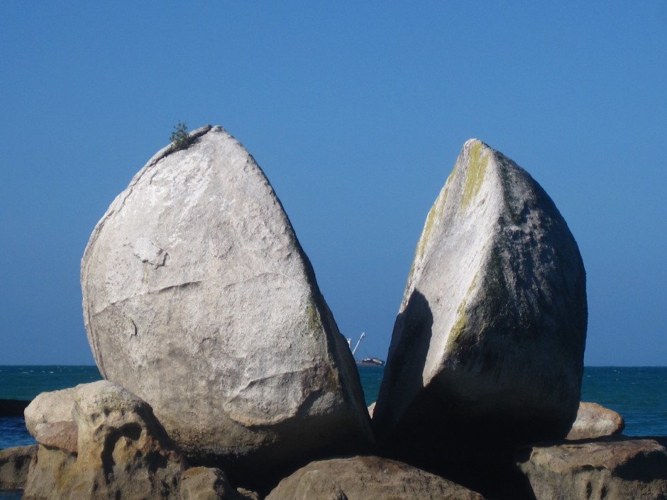
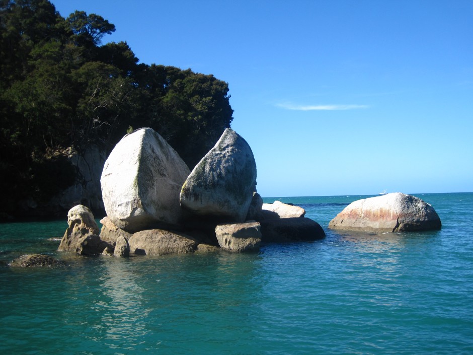
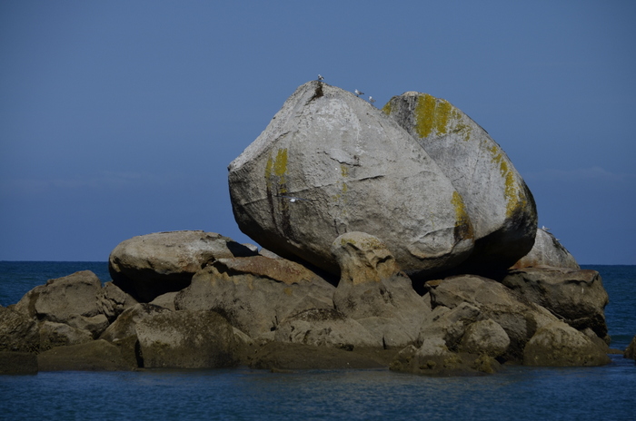
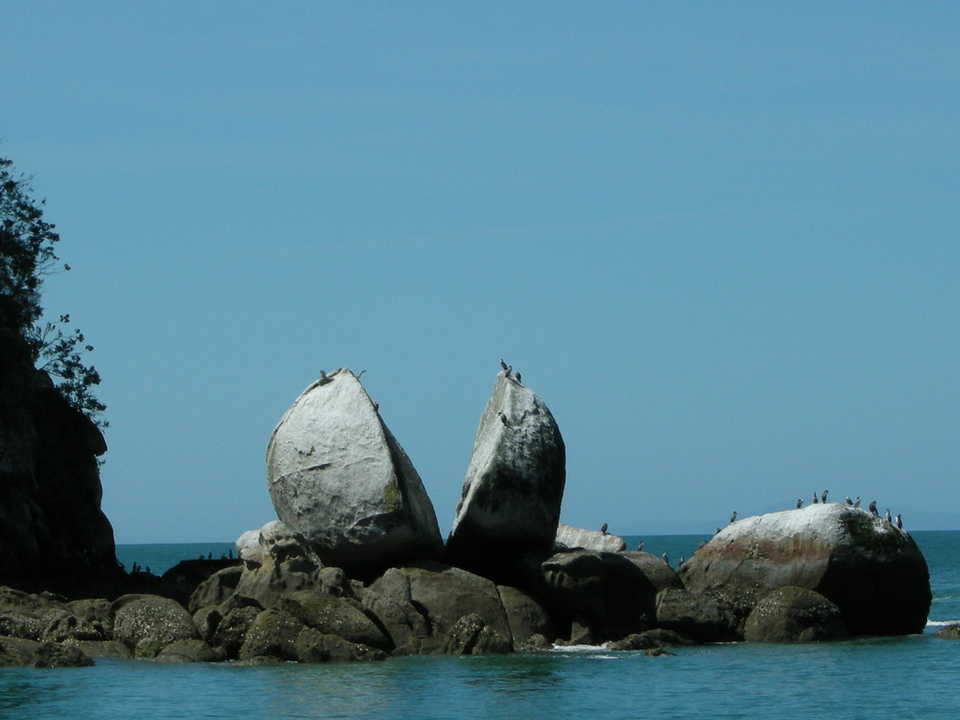
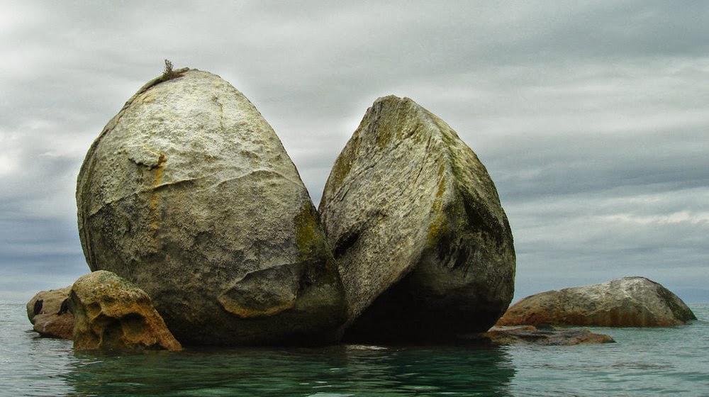
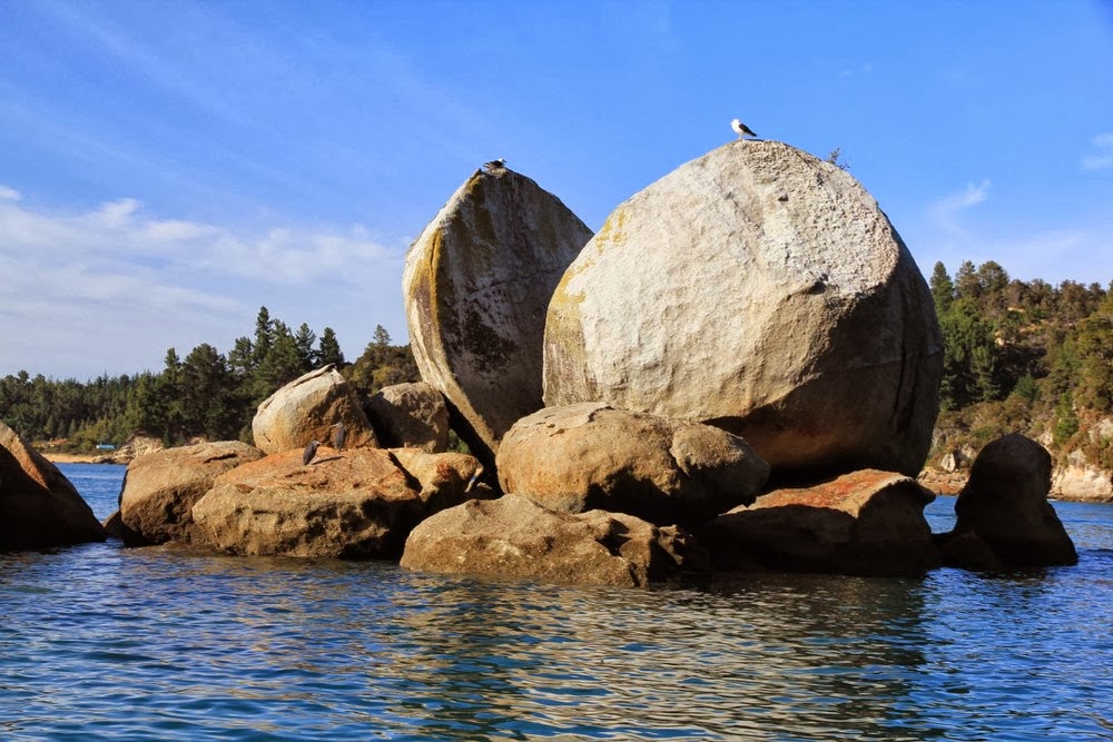
Split Apple Rock “Tokangawhā” is a geological rock formation in The Tasman Bay off the northern coast of the South Island of New Zealand.
Made of granite, it is in the shape of an apple which has been cut in half. It is a popular tourist attraction in the waters of the Tasman Sea approximately 50 metres off the coast between Kaiteriteri and Marahau.
The rock sits in shallow water at low tide and is accessible by wading. It is also a point of interest for the many tourist boats and pleasure craft which operate along the shores of the Abel Tasman National Park.
The cleft to produce two sides of the ‘apple’ was a natural occurrence. It is unknown when this happened and therefore the cleaving of the rock has attracted mythological explanations.
The name Split Apple Rock was made official in 1988, and was officially altered to Tokangawhā / Split Apple Rock in August 2014.
The mountain rises 8.6 kilometers, or roughly 5 miles, above the volcanic plain. Io is home to some of the highest mountains in the solar system, including some that tower 10 miles high, far higher than any mountain on Earth. Credit: NASA/JPL/University of Arizona
Mountains aren’t the first thing that hit you when you look at images of Jupiter’s innermost moon, Io. But once you absorb the fact that the moon is slathered in sulfurous lava erupted from 400 active volcanoes, you might turn your attention to scattered bumps and lumps that turn out, on closer inspection, to be Io’s version of mountains.There are about 100 of them, and they don’t look anything like the low lying volcanoes.
They also don’t look like mountains on our home world. While we favor majestic ranges stretching from horizon to horizon, the mountains on Io are isolated peaks of great height that jut up out of nowhere. From space, they look rather like the blocky chips in the fancier kind of chocolate chip cookie.
For planetary geophysicists like William McKinnon, professor of earth and planetary science in Arts & Sciences at Washington University in St. Louis, the mountains of Io are an intriguing puzzle. By what process consistent with everything that is known about Io could these bizarre mountains have formed?
Since Io buries the evidence of its tectonic processes under a continually refreshed coating of lava (adding 5 inches a decade), the scientists have turned increasingly to computer simulations to solve the problem. In the May 16 online advance issue of Nature Geoscience, McKinnon and Michael T. Bland, a research space scientist at the USGS Astrogeology Science Center in Flagstaff, Ariz., publish a computer model that is able to make numerical mountains that look much like the jutting rock slabs on Io.
Putting the squeeze on
“The planetary community has thought for a while that Io’s mountains might be a function of the fact that it is continuously erupting lava over the entire sphere,” McKinnon said. “All that lava spewed on the surfaces pushes downward and, as it descends, there’s a space problem because Io is a sphere, so you end up with compressive forces that increase with depth.”
McKinnon and his former student, Paul Schenk, now at the Lunar and Planetary Institute in Houston, wrote a paper explaining this hypothesis in 2001.
The numerical experiment described in Nature Geoscience tests this hypothesis through simulation. “People have been squeezing planetary interiors forever to see what happens,” McKinnon said, “but we’re applying the squeeze differently, because on Io compression increases with depth; the surface is not in compression. We thought we could mimic this by beveling in the edges of a box, squeezing it as you might an accordion.
The simulations show that the strain localizes to a single fracture, or fault, that starts deep in the lithosphere and rips through the rock all the way to the surface. When it breaches the surface, it actually overshoots, forming a scarp, or cliff, and stretching the surface of the overhanging block.
“It’s a neat demonstration of how things might actually work,” McKinnon said.
It might explain, for example, why there are often recent eruptions near mountains.
“The compressive forces deep in the crust are incredibly high,” Mckinnon said. “When these faults breach the surface, those forces are released, and the entire stress environment around the fault changes, providing a pathway for magma to erupt.”
The model might also explain why the mountains are associated with shallow, irregular depressions called patera. “When the stress environment changes,” McKinnon said, “a magma chamber can form at midlevel in the crust. When this magma surfaces along the fault, the crust above the chamber collapses, forming the patera.”
The model of mountain building also explains some of the “extensional” tectonic features on Io, such as “pull apart” mountains. These are mountains that have split in two parts that have shifted with respect to one another.
It might even explain a subtle feature of Io: the anti-correlation between mountains and volcanoes.
“If you look at a big map of Io,” McKinnon said, “there are concentrations of mountains and concentrations of volcanoes, and they kind of nest into one another. Even though mountains and volcanoes are often found together, if you look at all of the mountains and all of the volcanoes, they’re anti-correlated. It’s a peculiarity of Io.”
Why might this be? It’s not just the increasing weight of the overlying lava that puts the deep crust in compression McKinnon said, but also the increasing temperature. “Heating at depth causes the rocks to want to expand, and since there’s no room to expand, you again get compressive forces,” he said.
As long as the volcanoes are erupting, they carry this heat away and thermal stresses are low, reducing the likelihood of mountain formation. But if volcanism stops, the crust heats up, thermal stresses increase, and mountain formation becomes more likely.
Was Earth once like Io?
If all of this seems very alien, it is. “It’s a novel mountain-forming mechanism that we don’t see elsewhere in the solar system,” McKinnon said.
“But the same kind of thing could have happened on Earth, when it was very young and entirely covered by a shallow ocean,” McKinnon said.
“Because there was still lots of volcanism, mountains like those on Io might have burst through the ocean. They might have been the first emergent land on Earth,” McKinnon said.
So Io might be a time portal to the early Earth.
Reference:
“Mountain building on Io driven by deep faulting,” Nature Geoscience, published online May 16, 2016. DOI:10.1038/ngeo2711 This work was supported by NASA’s Planetary Geology and Geophysics Program (NNX11AP16G) and Solar System Workings Program (NNH15AZ801).
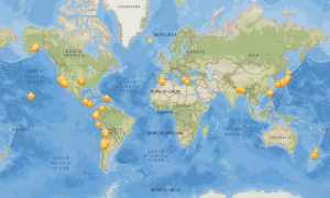
A map of the 121 earthquakes that MyShake users have recorded since the app’s release in February 2016. They range in magnitude form 2.5 to 7.8. Credit: Berkeley Seismological Laboratory
UC Berkeley scientists are releasing a Japanese version of an Android app that crowdsources ground-shaking information from smartphones to detect quakes and eventually warn users of impending jolts from nearby quakes.
The app, called MyShake, will be publicly available on Sunday, May 22 (Tokyo time), through the Google Play Store, which can be accessed via the MyShake website. It runs in the background and draws little power, so that a phone’s onboard accelerometers can record local shaking any time of the day or night. For now, the app only collects information from the accelerometers, analyzes it and, if it fits the vibrational profile of a quake, relays it and the phone’s GPS coordinates to the Berkeley Seismological Laboratory in California for analysis.
Since it was first released in English on Feb. 12, 2016, more than 170,000 people have downloaded the app from around the world, and on any given day 11,000 phones provide data to the system. In these three months, the network has recorded earthquakes in Chile, Argentina, Mexico, Morocco, Nepal, New Zeland, Taiwan, Japan and across North America, including induced earthquakes in Oklahoma. The system has recorded earthquakes as small as magnitude 2.5 and as large as the April 16, 2016, magnitude 7.8 earthquake in Ecuador.
Once enough people are using the app and the bugs are worked out, UC Berkeley seismologists plan to use the data to warn people miles from ground zero that shaking is rumbling their way.
“We think MyShake can make earthquake early warning faster and more accurate in areas that have a traditional seismic network, such as Japan, and can provide life-saving early warning in countries that have no seismic network,” said Richard Allen, the leader of the app project, director of the Berkeley Seismological Laboratory and a professor and chair of UC Berkeley’s Department of Earth and Planetary Sciences.
Allen will give an invited talk about the MyShake app and an early-warning system called ShakeAlert for the West Coast of the United States on Sunday morning, May 22, the opening day of the annual meeting of the Japan Geoscience Union. The meeting, held jointly with the American Geophysical Union, takes place at the Makuhari Messe convention center in Chiba, outside of Tokyo.
“In my opinion, this is cutting-edge research that will transform seismology,” said UC Berkeley graduate student Qingkai Kong, who developed the algorithm at the heart of the app. “The stations we have for traditional seismology are not that dense, especially in some regions around the world, but using smartphones with low-cost sensors will give us a really good, dense network in the future.”
Spanish and Chinese versions of the app are planned for the future, as is MyShake for the iPhone.
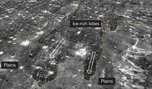
A 250-kilometre- long lobe of dark material might be the remnants of a tsunami that hit when Mars’ climate was cold enough to freeze the water into an ice-rich slush that crept across the landscape. Credit: Alexis Rodriguez
Some 3.4 billion years ago, giant meteoroids slammed into a frigid ocean covering Mars’s northern hemisphere. The impacts kicked up enormous waves that raced across the water and swamped the shoreline, research suggests.
On the scale of planetary catastrophes, such tsunamis would have dwarfed most Earthly ones. “Imagine this enormous red wave coming towards you, up to 120 metres high,” says Alexis Rodriguez, a Mars researcher at the Planetary Science Institute in Tucson, Arizona. “It would have been pretty spectacular.”
Rodriguez and his colleagues mapped traces of two of these tsunamis. They describe the findings in Scientific Reports.
If the idea stands up to further scrutiny, it may help resolve longstanding arguments about whether Mars had an ancient northern ocean. As evidence, some scientists point to what they call the remains of a shoreline, like a bathtub ring left behind when the water drained away. But the purported shoreline isn’t visible everywhere that it should be.
Mega-tsunamis could have wiped away some of that shoreline, happening as often as every 3 million years or so, Rodriguez says.
Wave function
Researchers have previously suggested tsunamis on Mars. A 2010 study calculated that high-energy waves should have left an imprint on the proposed Martian shoreline. A 2014 paper simulated how fast and how tall such waves might have moved — up to 20 metres a second as they rushed outward from the impact site, and up to 120 metres high when they reached the shore.
Rodriguez began thinking about Martian tsunamis after visiting the eastern coast of Japan in 2011, which had been devastated by a tsunami generated by a magnitude-9 earthquake. His team grew to include some top Martian geology experts.
The group zeroed in on a region on Mars where the highlands known as Arabia Terra bump up against the lowlands of Chryse Planitia — a place where the waters of an ancient ocean might have lapped at the shoreline. Using imagery from several Mars-orbiting spacecraft, Rodriguez’s group identified two particular geological formations that they say formed during two different tsunamis.
The first, older formation looks as if an enormous wave had rushed up onto the edge of the highlands, dropping boulders as big as 10 metres across. The water then drained back down into the ocean, leaving channels cut through the freshly deposited debris.
Then, millions of years passed. Temperatures dropped and glaciers crept across the landscape, scouring deep valleys. Finally, a second impact-generated tsunami came rushing again towards the shore. “But this time it is different,” Rodriguez says.
Because the climate was so much colder, the tsunami moved over the landscape like an icy slurry. It froze before it had a chance to wash back into the ocean, leaving dense lobes of frozen debris on the ground.
The new study is consistent with earlier ideas about how these Martian features formed, says Timothy Parker, a planetary scientist at the Jet Propulsion Laboratory in Pasadena, California, who originally came up with the idea of a northern Martian ocean. In previous work he described the backwash channels as forming when big waves washed up on a beach and drained back down again. “Though I didn’t specifically talk about tsunamis in my interpretations, the implication of scale was certainly there,” he says.
Iced out
The icy-looking lobes are particularly exciting, says James Dohm, a planetary scientist at the University Museum of the University of Tokyo. Even as the ocean eventually froze out and died, the tsunami deposits remained untouched by wind or other types of erosion for more than 3 billion years. (Dohm adds that he would have liked to have witnessed the Mars tsunamis, preferably from a high ridge and without an astronaut helmet blocking his vision.)
Rodriguez is now looking for evidence of tsunamis in other parts of Mars, as well as analogues on Earth that could help him to understand them better. One area of interest is a group of small craters near the shoreline that could have been drenched by the tsunami, and then trapped that water for millions of years. Such isolated pockets of water could have been places for Martian life to evolve, if it ever existed, Rodriguez says.
This summer, he hopes to travel to Tibet to study high, cold mountain lakes that may give him a glimpse into those long-ago Martian craters.
Note: The above post is reprinted from materials provided by Nature.
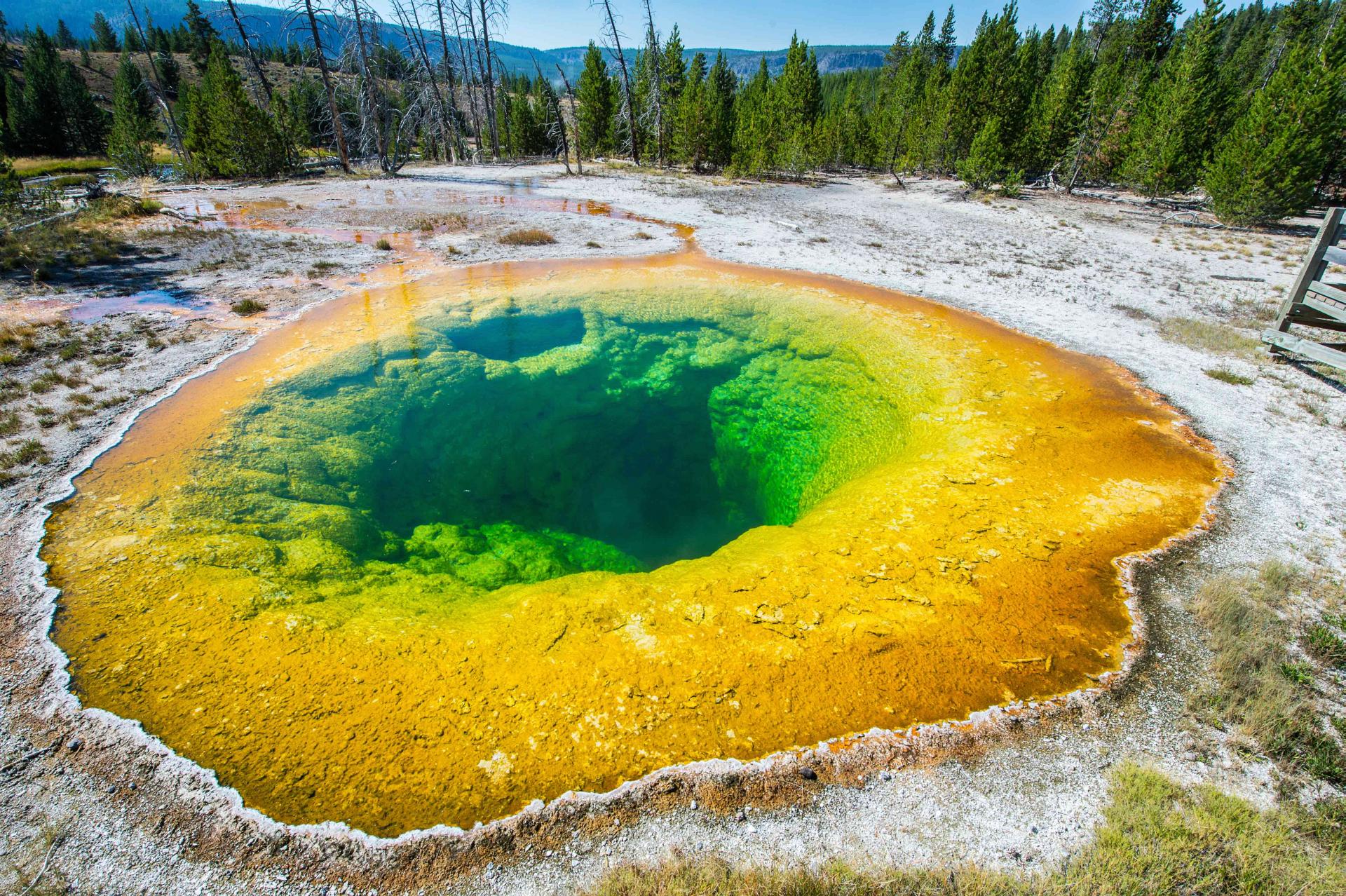
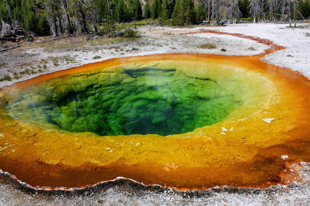
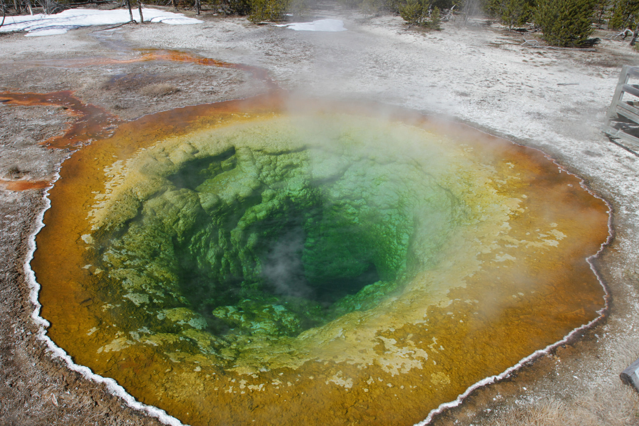
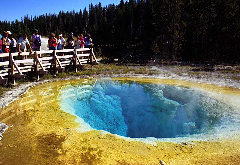
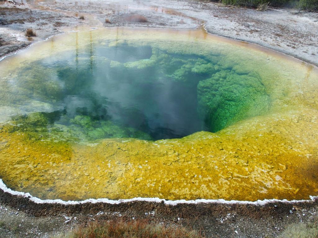
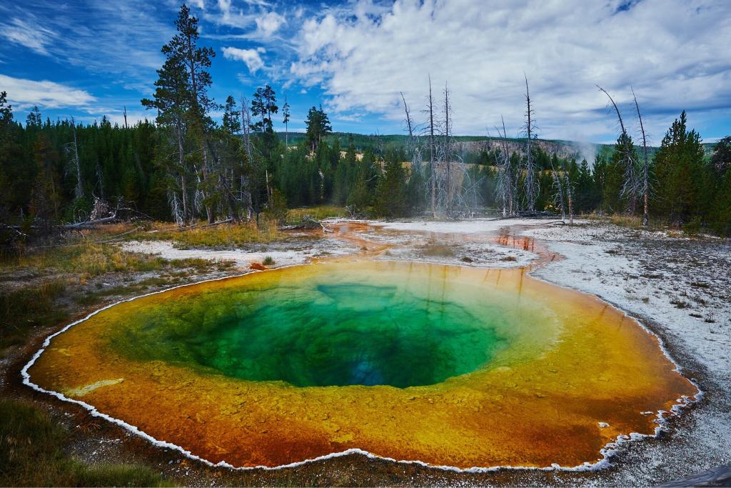
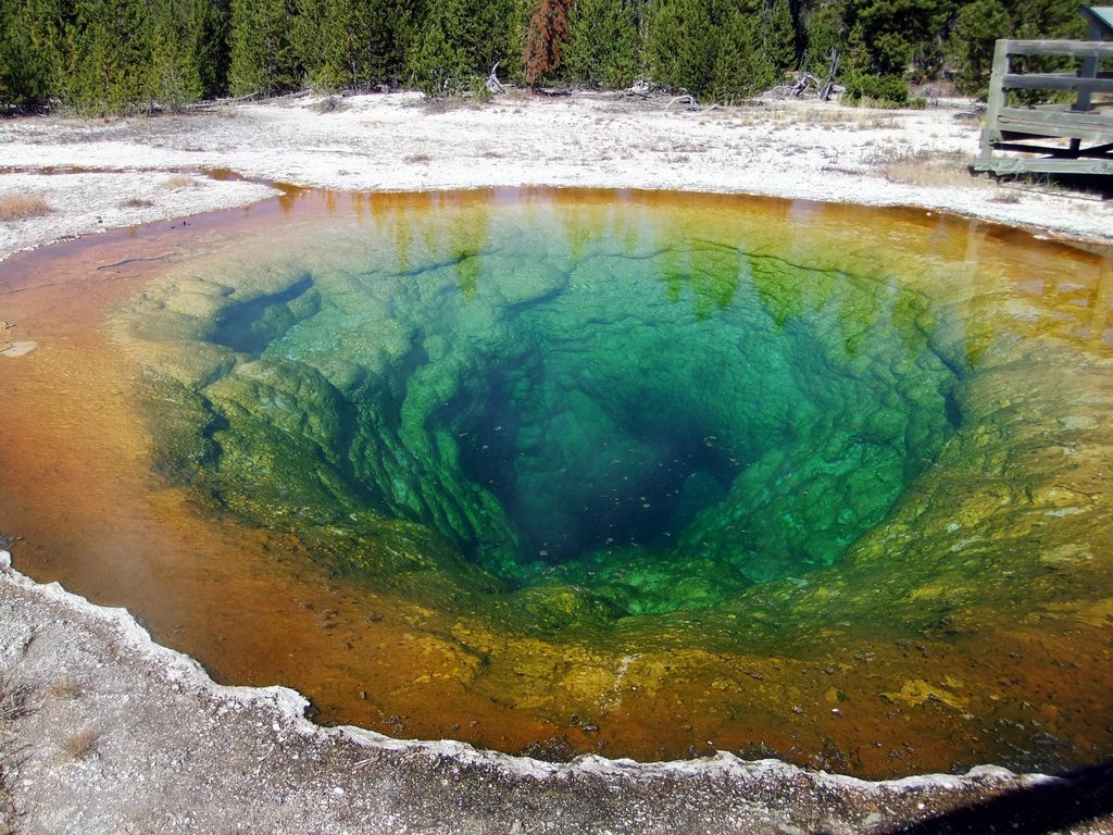
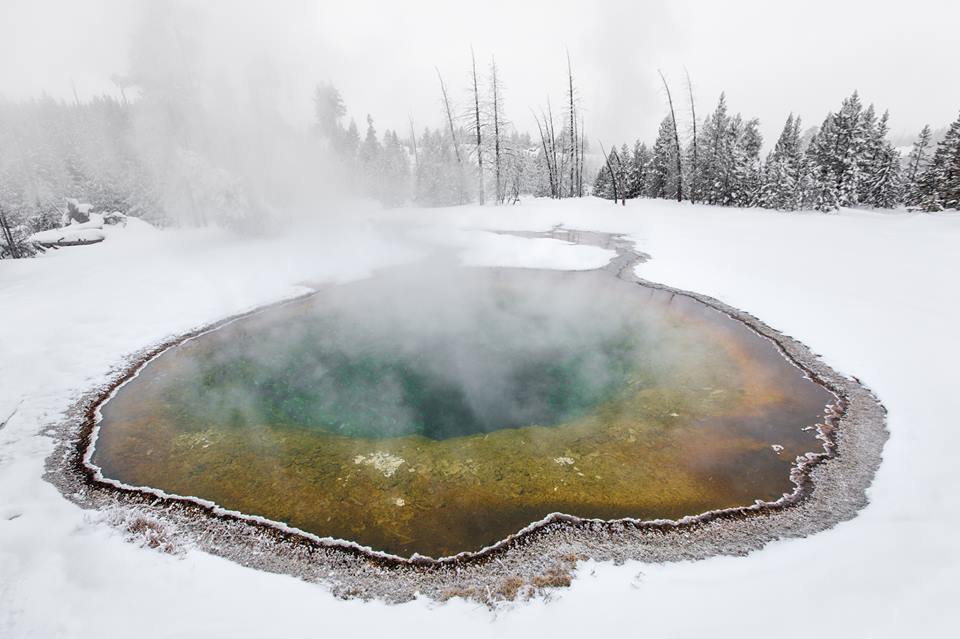
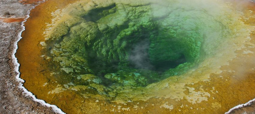
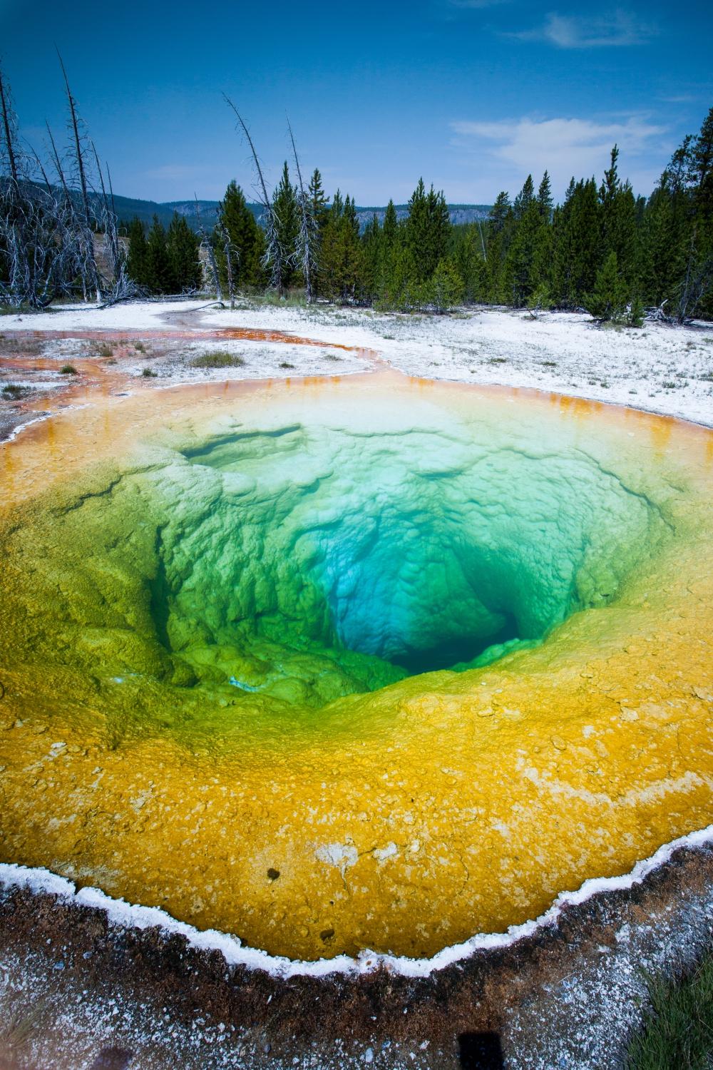
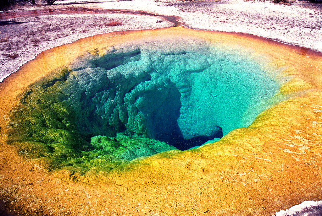
Morning Glory Pool is a hot spring in the Upper Geyser Basin of Yellowstone National Park in the United States.
History
The pool was named by Mrs E. N. McGowan, wife of Assistant Park Superintendent, Charles McGowan in 1883. She called it “Convolutus”, the Latin name for the morning glory flower, which the spring resembles. By 1889, the name Morning Glory Pool had become common usage in the park. Many early guidebooks called this feature Morning Glory Spring.
Composition
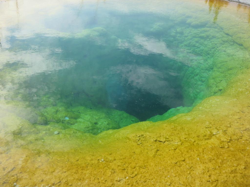
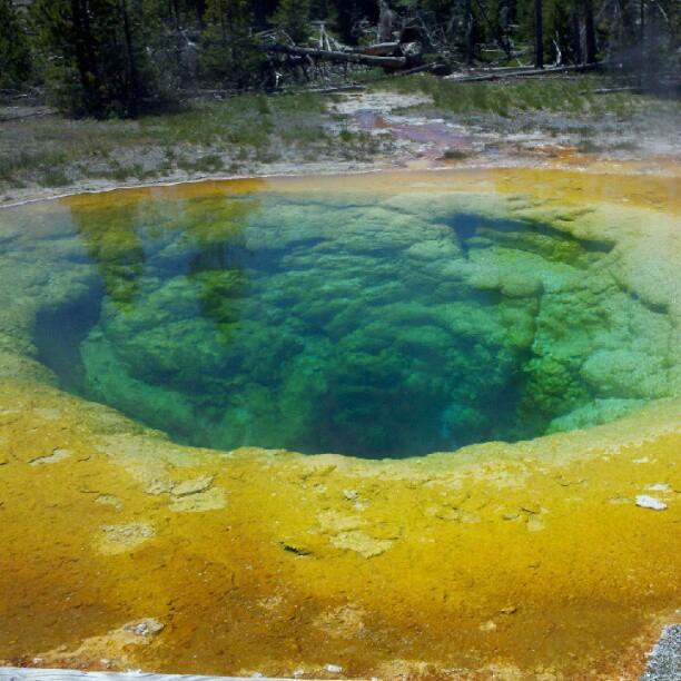
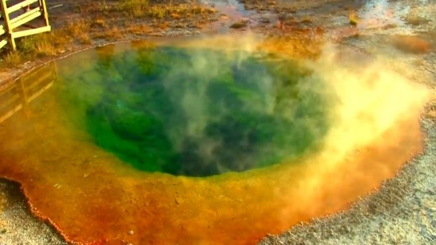
The distinct color of the pool is due to bacteria which inhabit the water. On a few rare occasions the Morning Glory Pool has erupted as a geyser, usually following an earthquake or other nearby seismic activity.
Several entryways have been clogged due to objects being thrown in by tourists, reducing the hot water supply, and in turn altering the overall appearance of the pool. Several attempts by park officials to artificially induce eruptions to clear the pool of debris and clear blocked entryways have been met with mixed results. An interpretive sign, placed near the pool by the park service, discusses the damage caused by ignorance and vandalism and suggests that Morning Glory is becoming a “Faded Glory.”
The anatomy of hydraulic fracturing. A pump truck injects fluid and proppant into a horizontally drilled well. The fluid fractures the formation and proppant holds these fractures open while natural gas flows out. Credit: Oregon State University
What is Hydraulic Fracturing?
Oil and natural gas, which are hydrocarbons, reside in the pore spaces between grains of rock (called reservoir rock) in the subsurface. If geologic conditions are favorable, hydrocarbons flow freely from reservoir rocks to oil and gas wells. Production from these rocks is traditionally referred to as “conventional” hydrocarbon reservoirs. However, in some rocks, hydrocarbons are trapped within microscopic pore space in the rock. This is especially true in fine-grained rocks, such as shales, that have very small and poorly connected pore spaces not conducive to the free flow of liquid or gas (called low- permeability rocks). Natural gas that occurs in the pore spaces of shale is called shale gas. Some sandstones and carbonate rocks (such as limestone) with similarly low permeability are often referred to as “tight” formations. Geologists have long known that large quantities of oil and natural gas occur in formations like these (often referred to as tight oil or gas). Hydraulic fracturing can enhance the permeability of these rocks to a point where oil and gas can economically be extracted.
Hydraulic fracturing (also known colloquially as “fracing,” or “fracking,”) is a technique used to stimulate production of oil and gas after a well has been drilled . It consists of injecting a mixture of water, sand, and chemical additives through a well drilled into an oil- or gas-bearing rock formation, under high but controlled pressure. The process is designed to create small cracks within (and thus fracture) the formation, and propagate those fractures to a desired distance from the well bore by controlling the rate, pressure, and timing of fluid injection. Engineers use pressure and fluid characteristics to restrict those fractures to the target reservoir rock, typically limited to a distance of a few hundred feet from the well. Proppant (sand or sometimes other inert material such as ceramic beads) is carried into the newly formed fractures to keep them open after the pressure is released and allow fluids (generally hydrocarbons) that were trapped in the rock to flow through the fractures more efficiently. Some of the water/chemical/proppant fracturing fluids remain in the subsurface. Some of this fluid mixture (called “flowback water”) returns to the surface, often along with oil, natural gas, and water that was already naturally present in the producing formation. This natural formation water is known as “produced water” and much of it is highly saline . The hydrocarbons are separated from the returned fluid at the surface, and the flowback and produced water is collected in tanks or lined pits. Handling and disposal of returned fluids has historically been part of all oil and gas drilling operations, and is not exclusive to wells that have been hydraulically fractured. Similarly, proper well construction is an essential component of all well-completion operations, not only wells that involve hydraulic fracturing. Well completion and construction, along with fluid disposal, are inherent to oil and gas development, and are specifically addressed in this paper because of concern about them and their relationship to hydraulic fracturing.
Hydraulic fracturing of shales and other tight rocks typically is through horizontal or directional (non-vertical) drilled wells which typically involve longer boreholes and much greater volumes of water than conventional oil and gas wells.
Hydraulic Fracturing’s History and Role in Energy Development
Hydraulic fracturing has been commercially applied since the 1940s. Over a million wells in the U.S. have been subjected to hydraulic fracturing, most of them conventional vertical oil and gas wells . Hydraulic fracturing became even more important in the 1990s, when improved technology allowed its application to horizontal wells in developing tight gas and oil reservoirs, particularly for shales. The technological combination of hydraulic fracturing, the chemistry of the fracturing fluid, and the use of horizontal wells is rapidly evolving. Traditional wells are drilled vertically (usually several thousand feet) and penetrate only a few tens or hundreds of feet of the reservoir rock. Horizontal wells start vertically, but then at a kickoff point are directed laterally (or horizontally) within the reservoir rock. The horizontal legs of these wells may extend as much as 10,000 feet through a reservoir rock, thus accessing a far greater volume of the reservoir than a traditional vertical well that only taps one vertical thickness of the reservoir rock. This replaces the need for multiple, vertical wells spaced closely on the land surface to tap the same reservoir volume. Because multiple wells can be drilled from one horizontal well pad, this further decreases the total amount of land needed for the drilling platform (called the “footprint”) and subsequent surface production equipment, although a horizontal well pad is typically much larger than a traditional vertical well pad. Because horizontal wells have both a vertical and a horizontal leg, and more contact with the reservoir rock than a traditional vertical well, horizontal wells typically require a larger volume of water than traditional vertical wells. This may be due to larger volumes of oil produced and not just the hydraulic fracturing requirements; one study compared the ratio of water use to oil produced for two different shale plays and found it was within the typical range for vertical, conventional oil wells over their lifespans. In a horizontal well, hydraulic fracturing usually occurs sequentially in several stages along the horizontal well bore (these are sometimes referred to as “staged treatments”), generally 10 to 15 pumping intervals, and sometimes as many as 50. Hydraulic fracturing of each stage may last from 20 minutes to four hours to complete .
In the past three decades, hydraulic fracturing has been increasingly used in formations that were known to be rich in natural gas that was locked so tightly in the rock that it was technologically and economically difficult to produce. The application of hydraulic fracturing to tight sands revitalized old fields and allowed establishment of new fields. Subsequently, the application of hydraulic fracturing to shale opened up huge new areas to development, including the Marcellus Shale in the eastern U.S, the Barnett Shale in Texas, and the Fayetteville Shale in Arkansas. The rise in production of natural gas from these and other shale plays was dramatic, to the point that natural gas prices have dropped and become more stable. Natural gas has become a major source of electrical power, and the U.S. may become a net natural gas exporter, if markets and regulations are favorable.
While hydraulic fracturing has had a huge impact on natural gas production, the same techniques have been applied to oil fields, leading to increased production from formations such as the Bakken and Three Forks Formations in North Dakota and Montana, and the Eagle Ford Formation in Texas. U.S. oil production from tight formations grew rapidly over the past several years. Future growth projections are uncertain, as the industry is influenced by global demand, prices, a social license to operate, regulations, well production life spans, and technological improvements that increase the percentage of recoverable hydrocarbons.
Water Quality
Fluids used in hydraulic fracturing are a mixture of water, proppant, and chemical additives. Additives typically include gels to carry the proppant into the fractures, surfactants to reduce friction, hydrochloric acid to help dissolve minerals and initiate cracks, inhibitors against pipe corrosion and scale development, and biocides to limit bacterial growth. The exact mix of additives depends on the formation to be fractured. Chemical additives typically make up about 0.5% by volume of well fracturing fluids, but may be up to 2%. Some potential additives are harmful to human health, even at very low concentrations. Unless diesel is used, the fracturing fluids are not regulated by the Safe Drinking Water Act (SDWA). Underground disposal of oil and gas wastes, however, is regulated by the SDWA.
Potential pathways for the fracturing fluids to contaminate water include surface spills prior to injection, fluid migration once injected, and surface spills of flowback and produced water. Because the fracturing fluids are injected into the subsurface under high pressure, and because some of the fluids remain underground, there is concern that this mixture could move through the well bore or fractures created in the reservoir rock by hydraulic pressure, and ultimately migrate up and enter shallow formations that are sources of freshwater (aquifers). There is also concern that geologic faults, previously existing fractures, and poorly plugged, abandoned wells could provide conduits for fluids to migrate into aquifers.
The potential to contaminate groundwater due to hydraulic fracturing is an environmental risk being studied. At present, there have been possibly two confirmed cases of groundwater contamination caused directly by the hydraulic fracturing process; in one location the fractured rock is within 420 feet of the aquifer. One challenge is to distinguish natural contaminants that seep into groundwater unrelated to oil and gas development, from contamination due to oil and gas development. There often are no water quality samples prior to hydraulic fracturing to provide a baseline comparison.
For example, methane has been detected in some water wells in areas with oil and gas development. Some researchers suggested hydraulic fracturing may be responsible for methane in water wells in northeastern Pennsylvania and upstate New York, although leaky well casings is a more likely possibility. In some geologic settings, methane can naturally originate from gas-producing rock layers below and close to the aquifer and be unrelated to the deeper fractured zone. Analysis of the gas can be used to identify the origin of gas occurring in groundwater. In one study of drinking water wells near shale gas well sites in Pennsylvania and Texas, wells were sampled for hydrocarbon gas to determine if contamination had occurred.. The researchers concluded that contamination has locally occurred, and, for those wells with elevated gas levels, the fugitive gas appeared to have migrated from shallower rocks through cracks in the cement around the well (annulus), leaks in the well casing, or from other well failures, rather than from the artificial hydraulic fractures in the reservoir rock. An analysis of a large database on dissolved methane in domestic wells and proximity to pre-existing oil and gas wells in Pennsylvania indicated no statistically significant relationship, although the study had criticism for its industry support for the study.
There have been confirmed cases of groundwater contamination from improperly constructed, oil and gas wells. To protect groundwater, proper well design, construction, and monitoring are essential. During well construction, multiple layers of telescoping pipe (or casing) are installed and cemented in place, with the intent to create impermeable barriers between the inside of the well and the surrounding rock. It is also common practice to pressure test the cement seal between the casing and rock or otherwise examine the integrity of wells. Wells that extend through a rock formation that contains high-pressure gas require special care in stabilizing the well bore and stabilizing the cement or its integrity can be damaged. As with any mechanical device or barrier, failures can occur. There is significant variability in the estimated failure rates of the integrity of oil and gas wells. Local regulations, the technology, the geologic setting and the prevailing operational culture influence the well completion, abandonment and monitoring, and these evolve over time. Differences in the type and sizes of well integrity datasets adds to the challenge of generalizing well integrity failure rates.
The physical separation between the relatively shallow freshwater aquifer and the typically much deeper oil- and gas-producing rock layer provides protection to shallow aquifers. Typically there are thousands of feet of mostly low- to very low-permeability rock layers between an aquifer and oil or gas reservoir rocks that prevent fracturing fluids and naturally migrated hydrocarbons from reaching the aquifer. In areas where there is concern about faults, fractures, or plugged wells, various geophysical methods can be used to locate and avoid faults, although such surveys are time consuming and expensive. There is also renewed interest in the need to locate and plug abandoned or “orphaned” oil and gas wells, and unused water wells, as a further measure to protect near-surface aquifers. It will also be prudent to develop technologies to monitor deep groundwater. In some regions, identifying and properly plugging all the abandoned wells is a significant undertaking.
Proper storage and disposal of fracturing fluids and produced water is important to ensure that both surface water and groundwater are protected. Most fracturing fluids and produced water are re-injected into Class II wells drilled specifically for deep disposal, treated in wastewater treatment facilities, or recycled. Wastewater treatment facilities, designed primarily for municipal waste, can be overwhelmed with the volume and treatment of fracturing fluids and produced water; a number will not accept such waste. Disposal wells inject waste water deep into formations that originally produced the oil and gas, or into different formations that generally contain highly saline and otherwise unusable water. Water is generally co-produced in equal or larger volumes than petroleum throughout the life of a well. Fluid handling and disposal are important issues for all oil and gas activity. Appropriate management practices and regulatory oversight help assure that accidental leaks and spills are minimized.
Baseline water-quality testing, carried out prior to oil and gas drilling, helps to document the quality of local natural groundwater and may identify natural or pre-existing contamination, or lack thereof, before oil and gas activity begins. Without such baseline testing, it is difficult to know if contamination existed before drilling, occurred naturally, or was the result of oil and gas activity. Many natural constituents, including methane, elevated chlorides, and trace elements occur naturally in shallow groundwater in oil- and gas-producing areas and are unrelated to drilling activities. The quality of water in private wells is not regulated at the state or federal level, and many owners do not have their well water tested for contaminants. States handle contamination issues differently. For instance, Colorado and Ohio require baseline sampling of wells in oil- and gas-producing regions as part of its regulatory process. Pennsylvania places the presumptive burden of proof on oil and gas companies if groundwater contamination of drinking-water sources is found. In most states, however, such baseline sampling is not required.
Although there is little evidence of groundwater contamination due to hydraulic fracturing itself, there are still many questions about the risks to aquifers with the rapidly expanding industry developing tight oil and gas reservoirs using modern hydraulic fracturing techniques. There are few long term, peer-reviewed scientific studies. The U.S. Environmental Protection Agency’s (EPA) Scientific Advisory Board study Potential Impacts of Hydraulic Fracturing on Drinking Water Resources (projected to be finalized in 2016) will be an important contribution. Local baseline testing of groundwater quality prior to hydraulic fracturing operations can provide valuable data for later assessing claims of contamination.
Contamination risks to surface water during development of tight oil and gas plays has led to increased regulations in some U.S. states. Potential pathways for contamination include surface spills, waste disposal, and surface spreading of well cuttings. A study of the gas shale development in Pennsylvania documented increased chlorides downstream of the waste treatment plant and elevated total suspended solids downstream of shale gas wells. The elevated suspended solids appear related to the land clearing for the well pad, roads, and related infrastructure.
Water Use
Hydraulic fracturing, particularly when applied to horizontal wells, can use 13 million gallons or more water per well, though two to five million gallons is typical. However, the ratio of “water used” to “oil produced” in hydraulically fractured wells in the Eagle Ford Shale, Texas, and Bakken Shale, North Dakota, is on the low end of what is typically used in a conventional, vertical oil well over the life of the well. The study concluded that the higher water use reflects an increase in oil production, and not that hydraulic fracturing uses more water per unit of oil produced than conventional wells. Water used in oil and gas development is relatively small in comparison to other recurring uses. However, where drilling rates are high, and particularly in water-poor areas, water use for oil and gas development is significant. The U.S. EPA is studying the current and future potential competition between hydraulic fracturing and drinking water supplies in two basins, one humid (Susquehanna River Basin, Pennsylvania) and one semi-arid (Upper Colorado River Basin, Colorado). Water needs 30 years out are based on drilling trends, natural gas production, and population growth.
Drilling companies are working on improved methods to recycle water used in hydraulic fracturing, or to use saline water that is unsuitable for drinking. Many energy companies are treating and reusing produced and flowback water; the feasibility depends on economics, and the quantity, quality, and duration of water generated. Some companies are trying water-free, nonflammable propane fracking fluid. However, because of chemical mixing considerations and costs, freshwater continues to be the preferred and primary source of water for hydraulic fracturing in most areas. In December 2015, the Governor of Oklahoma formed a task force to find economic treatment and uses for the produced water.
Geology
Mechanics
Fracturing rocks at great depth frequently becomes suppressed by pressure due to the weight of the overlying rock strata and the cementation of the formation. This suppression process is particularly significant in “tensile” (Mode 1) fractures which require the walls of the fracture to move against this pressure. Fracturing occurs when effective stress is overcome by the pressure of fluids within the rock. The minimum principal stress becomes tensile and exceeds the tensile strength of the material. Fractures formed in this way are generally oriented in a plane perpendicular to the minimum principal stress, and for this reason, hydraulic fractures in well bores can be used to determine the orientation of stresses. In natural examples, such as dikes or vein-filled fractures, the orientations can be used to infer past states of stress.
Veins
Most mineral vein systems are a result of repeated natural fracturing during periods of relatively high pore fluid pressure. The impact of high pore fluid pressure on the formation process of mineral vein systems is particularly evident in “crack-seal” veins, where the vein material is part of a series of discrete fracturing events, and extra vein material is deposited on each occasion. One example of long-term repeated natural fracturing is in the effects of seismic activity. Stress levels rise and fall episodically, and earthquakes can cause large volumes of connate water to be expelled from fluid-filled fractures. This process is referred to as “seismic pumping”.
Dikes
Minor intrusions in the upper part of the crust, such as dikes, propagate in the form of fluid-filled cracks. In such cases, the fluid is magma. In sedimentary rocks with a significant water content, fluid at fracture tip will be steam.
Induced Seismicity
Induced seismicity is an earthquake caused by human activities. One way this can occur is from iInjection of fluids deep into the earth. The increase in underground disposal of produced and flowback water from oil and gas wells are associated with a large increase in triggered small and moderate earthquakes in some regions, such as central and northern Oklahoma . Oil and gas operations are responsible for two types of fluid injection: 1) injection of hydraulic fracturing fluids into the reservoir rock; and 2) disposal of waste fluids through deep well injection.
Hydraulic fracturing imparts pressures of several thousand pounds per square inch on reservoir rocks. The resulting fractures may extend several hundred feet away from the borehole, but generally no more than that due to physical and technological limitations on the hydraulic fracturing process. The hydraulic fracturing process creates very small seismic events or earthquakes. Such microseismicity is generally too small for humans to feel or to cause surface damage, although it can be detected by monitoring instruments that are designed to precisely determine where the fractures have propagated. A number of studies, including one by the National Academy of Sciences, have determined that hydraulic fracturing does not create a significant earthquake risk. Alberta and British Columbia, Canada, have had moderate earthquakes that appear related to the hydraulic fracturing process itself.
Disposal of large volumes of waste fluids produced from hydraulically fractured rocks through deep-well injection has been documented to produce small earthquakes, generally less than magnitude 2.0. However, in areas with high volumes and rates of injection into disposal wells, there have been dramatic increases in earthquakes magnitude 3.0 and greater. Horizontal wells that have been hydraulically fractured typically produce large volumes of waste fluids (produced and flowback water). Deep disposal of any fluids can trigger earthquakes. Most, although not all, of such earthquakes have occurred in areas of long-term or continuous injection of wastewater. Fluids injected near a subsurface fault may reduce the frictional resistance that keeps faults from slipping. These small movements allow energy already stored in brittle rock to be released in earthquakes. In some locations, sites of slowly accumulating forces in the earth resulting from natural geologic processes are already susceptible to seismic events (which is why it is referred to as “triggered seismicity”). The increase in pore pressure on stressed fault surfaces appears to be the main physical reason for injection-induced earthquakes in the central and eastern United States . Deep well injection of fluids has likely caused earthquakes in excess of magnitude 2.0 over the past several decades, including a magnitude 5.7 earthquake in 2011 in Oklahom and a sharp increase of earthquake frequency from 2012 to 2015 in Oklahoma. Kansas has also experienced a marked increase in seismic activity in the last two years, including the state’s largest earthquake recorded at magnitude 4.9 in November 2014. The potential for triggered seismicity with the increasing volume of wastewater disposal is unknown. States are implementing strategies to mitigate risks of induced seismicity associated with disposal injection wells. This includes a screening protocol to determine what response strategies may be appropriate. Mitigation actions can include changing the allowable rates and pressures of injection, partial plugback of the injection well, and stopping all injections and shutting the well.
Uses
Hydraulic fracturing is used to increase the rate at which fluids, such as petroleum, water, or natural gas can be recovered from subterranean natural reservoirs. Reservoirs are typically porous sandstones, limestones or dolomite rocks, but also include “unconventional reservoirs” such as shale rock or coal beds. Hydraulic fracturing enables the extraction of natural gas and oil from rock formations deep below the earth’s surface (generally 2,000–6,000 m (5,000–20,000 ft)), which is greatly below typical groundwater reservoir levels. At such depth, there may be insufficient permeability or reservoir pressure to allow natural gas and oil to flow from the rock into the wellbore at high economic return. Thus, creating conductive fractures in the rock is instrumental in extraction from naturally impermeable shale reservoirs. Permeability is measured in the microdarcy to nanodarcy range. Fractures are a conductive path connecting a larger volume of reservoir to the well. So-called “super fracking,” creates cracks deeper in the rock formation to release more oil and gas, and increases efficiency. The yield for typical shale bores generally falls off after the first year or two, but the peak producing life of a well can be extended to several decades.
While the main industrial use of hydraulic fracturing is in stimulating production from oil and gas wells, hydraulic fracturing is also applied:
To stimulate groundwater wells
To precondition or induce rock cave-ins mining
As a means of enhancing waste remediation, usually hydrocarbon waste or spills
To dispose waste by injection deep into rock
To measure stress in the Earth
For electricity generation in enhanced geothermal systems
To increase injection rates for geologic sequestration of CO2
Since the late 1970s, hydraulic fracturing has been used, in some cases, to increase the yield of drinking water from wells in a number of countries, including the US, Australia, and South Africa.
Economic effects
Hydraulic fracturing has been seen as one of the key methods of extracting unconventional oil and unconventional gas resources. According to the International Energy Agency, the remaining technically recoverable resources of shale gas are estimated to amount to 208 trillion cubic metres (208,000 km3), tight gas to 76 trillion cubic metres (76,000 km3), and coalbed methane to 47 trillion cubic metres (47,000 km3). As a rule, formations of these resources have lower permeability than conventional gas formations. Therefore, depending on the geological characteristics of the formation, specific technologies (such as hydraulic fracturing) are required. Although there are also other methods to extract these resources, such as conventional drilling or horizontal drilling, hydraulic fracturing is one of the key methods making their extraction economically viable. The multi-stage fracturing technique has facilitated the development of shale gas and light tight oil production in the United States and is believed to do so in the other countries with unconventional hydrocarbon resources.
The National Petroleum Council estimates that hydraulic fracturing will eventually account for nearly 70% of natural gas development in North America. Hydraulic fracturing and horizontal drilling apply the latest technologies and make it commercially viable to recover shale gas and oil. In the United States, 45% of domestic natural gas production and 17% of oil production would be lost within 5 years without usage of hydraulic fracturing.
U.S.-based refineries have gained a competitive edge with their access to relatively inexpensive shale oil and Canadian crude. The U.S. is exporting more refined petroleum products, and also more liquified petroleum gas (LP gas). LP gas is produced from hydrocarbons called natural gas liquids, released by the hydraulic fracturing of petroliferous shale, in a variety of shale gas that’s relatively easy to export. Propane, for example, costs around $620 a ton in the U.S. compared with more than $1,000 a ton in China, as of early 2014. Japan, for instance, is importing extra LP gas to fuel power plants, replacing idled nuclear plants. Trafigura Beheer BV, the third-largest independent trader of crude oil and refined products, said at the start of 2014 that “growth in U.S. shale production has turned the distillates market on its head.”
Some studies call into question the claim that what has been called the “shale gas revolution” has a significant macro-economic impact. A study released in the beginning of 2014 by the IDDRI concluded the contrary. It states that, on the long-term as well as on the short-run, the “shale gas revolution” due to hydraulic fracturing in the United States has had very little impact on economic growth and competitiveness. The same report concludes that in Europe, using hydraulic fracturing would have very little advantage in terms of competitiveness and energy security. Indeed, for the period 2030-2035, shale gas is estimated to cover 3 to 10% of EU projected energy demand, which is not enough to have a significant impact on energetic independence and competitiveness.
Hydrofracked shale oil and gas has the potential to alter the geography of energy production in the US. In the short run, in counties with hydrofracturing employment in the oil and gas sector more than doubled in the last 10 years, with spill-overs in local transport-, construction but also manufacturing sectors. The manufacturing sector benefits from lower energy prices, giving the US manufacturing sector a competitive edge. On average, natural gas prices have decreased by more than 30% in counties above shale deposits compared to the rest of the US. Some research has highlighted the negative effects on house prices for properties in the direct vicinity of fracturing wells. Local house prices in Pennsylvania decrease if the property is close to a hydrofracking gas well and is not connected to city water, suggesting that the concerns of ground water pollution are priced by markets.
Representative Image:Digital skull models of Erlikosaurus andrewsi, Stegosaurus stenops, and Plateosaurus engelhardti (from left to right) Credit: Stephan Lautenschlager
The first detailed study of a Stegosaurus skull shows that the dinosaur had a stronger bite than suspected, enabling it to eat a wider range of plants than other plant-eating dinosaurs with similarly shaped skulls.
A team of scientists from Bristol, London, Manchester and University of Birmingham compared the skull of ‘Sophie’, the Natural History Museum’s new Stegosaurus specimen, with two other dinosaurs, Plateosaurus and Erlikosaurus, which shared similar skull characteristics. Computer modelling at the University of Bristol showed that, despite looking very similar, the dinosaurs had different biting abilities.
Although the three dinosaurs existed in different time periods and locations and had very differently shaped bodies, all three had similar-looking skulls: a large low snout, feeble peg-shaped teeth, and a scissor-like jaw action only capable of moving up and down. All three ate mainly or exclusively plants.
Until now, it has been assumed that the dinosaurs probably had similar biting abilities and therefore ate similar types of plants. But the research reveals that it can be a trap to assume that because a set of dinosaurs shared a set of similar features, they all operated in the same way – function does not necessarily follow form.
As Prof. Paul Barrett, Merit Researcher at The Natural History Museum explains: ‘Our key finding really surprised us: we expected that many of these dinosaur herbivores would have skulls that worked in broadly similar ways. Instead we found that even though the skulls were fairly similar to each other in overall shape, the way they worked during biting was substantially different in each case.’
Stegosaurus lived around 150 million years ago and needed to eat a lot of plants to sustain its large size. As grasses did not exist then, it would have fed on plants such as ferns and horsetails. However the research indicates that it had a much higher bite force than anyone had suspected, enabling it to a wider range of plants than previously thought.
As Barrett, leader of the research team, comments: ‘Far from being feeble, as usually thought, Stegosaurus actually had a bite force within the range of living herbivorous mammals, such as sheep and cows.’
This wider range of plants means that scientists need to reconsider how Stegosaurus fitted into its ecological niche. For example it may have had a role in spreading the seeds of cycads – woody ever green plants that were abundant in the time of the dinosaurs and whose seeds are contained in large cones.
Dr David Button, from the University of Birmingham’s School of Geography, Earth and Environmental Sciences, said: ‘The extra information provided by computing modelling is invaluable. Although we can tell roughly what a dinosaur ate from the shape of its teeth and jaws, the differences highlighted by this study indicate that the biology and ecology of these animals is more complex than we previously thought. As we study the lives of dinosaurs in greater detail, they continue to surprise us.’
Lead author Dr Stephan Lautenschlager, a post-doctoral researcher at the University of Bristol’s School of Earth Sciences, employed digital models and computer simulations to analyse the dinosaurs’ bites, using data from 3D scans of the skulls and lower jaws. He used engineering software to give the skulls the material properties that would match as closely as possible to the real thing, for example, using data on crocodile teeth to model those of the dinosaurs. By attaching muscles to the models, he was able to examine the forces that the jaws could produce and the subsequent stresses on the skulls.
As computer power increases and software becomes more available, Lautenschlager thinks that we will see more modelling used in dinosaur research: ‘Using computer modelling techniques, we were able to reconstruct muscle and bite forces very accurately for the different dinosaurs in our study. As a result, these methods give us new and detailed insights into dinosaur biology – something that would not have been several years ago.’
Reference:
Lautenschlager, S. Brassey, C. A., Button, D. J., Barrett, P. M.. Decoupled form and function in disparate herbivorous dinosaur clades. Sci. Rep. 6, 26495; DOI: 10.1038/srep26495
Scientists studying deltas show how they may be able to predict where destructive changes in a river’s course may occur.
A delta forms when a river meets a sea or ocean. Deltas are extremely fertile for crops, and home to over half billion people and several mega-cities.
An avulsion – where the flow of water through a delta changes its course – can be sudden and unpredictable, often catching communities off-guard. When it happens, the river floods the neighbouring areas, threatening livelihoods and destroying valuable farming land.
The team suggest that their study could lead to a new method for predicting where avulsions may occur. The researchers say many river delta systems are drowning because of rising sea levels. This could push avulsions farther upstream placing more and more communities in jeopardy and making an avulsion predicting tool even more vital.
Many deltas are built over several thousands of years when sand and soil are deposited in huge leaf-shaped patterns called lobes. When an avulsion occurs the river changes its course and a new lobe is constructed.
The team constructed a replica of this type of river delta in the lab, which was over two metres long. They subjected it to different flooding conditions that would normally happen over a time-scale of several hundreds to thousands of years. Through their experiments they were able to confirm that the constant cycle of flooding was a key factor that contributes to locating where the next avulsion is likely to occur.
Dr Vamsi Ganti from Imperial’s Department of Earth Science and Engineering carried out the study with his colleagues while at California Institute of Technology in the USA. It is published in the journal Science Advances.
Dr Ganti said: “Around the world we see deltas under constant pressure. The Mississippi River delta for instance, is drowning at an alarming rate, and has lost around 5,000 square kilometres of land since the 1930s. So, understanding more about avulsions is vital in protecting the people and ecosystems that deltas support, and also mitigating land loss.”
“Avulsions are often thought of as the ‘earthquakes’ of deltas because of the damage they wreak. Sudden and unpredictable changes in the course of a river can rapidly flood neighbouring land, meaning that people often have to abandon their communities before they are swallowed by the river system.
“Our research confirms the factors that make these avulsions occur, which could ultimately help people around the world make their communities more secure.”
Scientists had previously observed that lobes always reach a uniform length that is characteristic to each delta. They developed a formula that showed the lobe length is related to the gradient and the depth of the river running through the delta.
The researchers in the study discovered that the uniform lobe length only occurs when their delta in the lab was subjected to floods. This causes the lobe to reach its uniform length, which then triggered an avulsion. By bringing together all their findings the researchers are working towards a method for predicting where avulsions may occur on many of the deltas in the world.
The researchers also think their results could be used to understand how river delta systems are built on other planets that once had water such as Mars. This could help scientists learn more about past oceans and seas on other planets.
Video
Reference:
“Experimental river delta size set by multiple floods and backwater hydrodynamics,” Science Advances, DOI: 10.1126/sciadv.1501768
A team of National Science Foundation (NSF)-supported researchers at the Virginia Polytechnic Institute and State University (Virginia Tech) discovered new evidence about how the Earth’s magnetic field interacts with solar wind, almost as soon as they finished installing six data-collection stations across East Antarctic Plateau last January.
Their findings could have significant effects on our understanding of space weather. Although invisible to the naked eye, space weather can have serious, detrimental effects on modern technological infrastructure, including telecommunications, navigation, and electrical power systems.
The researchers for the first time observed that regardless of the hemisphere or the season, the polar ionosphere is subject to a constant electrical current, produced by pressure changes in the solar wind.
“This finding is a new part of the physics that we need to understand and work with,” said Robert Clauer, a professor in Virginia Tech’s Bradley Department of Electrical and Computer Engineering. “It’s a bit of a surprise, because when you have a current, you usually expect a voltage relationship, where resistance and current are inversely related—high resistance equals small current; low resistance equals large current.”
These space weather observations allow researchers to watch how the behavior of the sun and the solar wind—an unbroken supersonic flow of charged particles from the sun—changes over time and how the Earth’s magnetic field responds to solar wind variations. The observations help build a detailed, reliable model of space weather.
They hope that eventually space weather forecasting will become as reliable as today’s winter storm warnings.
The project to develop and deploy these autonomous data-collection stations in the Antarctic, funded by a $2.7 million NSF award, has progressed over a seven-year period. NSF manages the U.S. Antarctic Program, through which it supports researchers nationwide, provides logistical support to the research and operates three year-round stations in Antarctica.
Clauer and his team designed and hand-built six autonomous data-collection stations and installed them piece-by-piece near the geographic South Pole for initial testing. Following successful testing, the autonomous data-collection stations were placed along the 40-degree magnetic meridian (longitude), deep in the southern polar cap areas under the auroras. The stations, located in the harsh environment of the remote East Antarctic Plateau, are the Southern Hemisphere counterpart to a magnetically similar chain in Greenland.
Clauer and his Magnetosphere-Ionosphere Science team have been monitoring the electric current systems in the magnetosphere—specifically currents that connect to the ionosphere. During the summer in the Northern Hemisphere, there is more direct sunlight on the atmosphere, which means more atoms are ionized. This phenomenon creates a highly conductive ionosphere in the summer months and a poorly conductive one in the winter.
“The solar wind interacts with Earth’s magnetic field in a manner similar to a fluid, but an electrically conducting fluid,” Clauer said.
A chain of data-collection stations in Greenland allowed researchers to take measurements in the Northern Hemisphere. Until recently, these data were divided into summer and winter, and the information gathered during the winter months was used to approximate what was happening in the Southern Hemisphere during the northern summer.
“We didn’t have a full picture of what was happening in the space environment because we could only observe one hemisphere, but magnetic field lines are connected to both hemispheres,” said Clauer. “It was important that we look at them simultaneously.”
The stations run autonomously and are powered by solar cells in the months-long Antarctic summer, and by lead-acid batteries during winter. The stations contain a collection of instruments, including a dual-frequency GPS receiver that tracks signal changes produced by density irregularities in the ionosphere, and two kinds of magnetometers that measure the varying strength and direction of magnetic fields. The data is transmitted to Blacksburg, Virginia, via Iridium satellites.
Clauer’s team will continue collecting information from both sets of data stations. They hope to operate throughout the 11-year solar activity cycle, depending on snow accumulation.
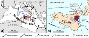
Fig. 1. (a) Tectonic map showing the geodynamic framework of the Mediterranean region. (b) Main structural features of Sicily and location of the volcanic areas studied in the V3 Project. Credit: Modified from Billi et al. [2006]A new project elucidates the relationships between tectonics and volcanic systems and how they influence hazards on Italy’s Mount Etna and Vulcano and Lipari islands.
Mount Etna and the Aeolian Islands in southern Italy represent ideal natural laboratories to study how magma and tectonics interact in active volcanic zones and their associated hazards. The geodynamic context of both areas is characterized by a tectonic compression running north and south, related to the convergence of the African and Eurasian plates in the central Mediterranean (Figure 1). This compression creates a cluster of volcanoes, some of the most active in Europe.
The region’s proximity to major urban centers is a double-edged sword. Researchers have little trouble visiting volcanoes to study how tectonics influence volcanic plumbing. At the same time, this proximity presents hazards to inland communities and those on nearby shores.
To take advantage of this natural laboratory and to help protect people living nearby, several branches of Italy’s government research community established the V3 Project—so named because it is project number 3 of the Italian Civil Protection Department’s Volcanological Research Program. Data collection for the project ran from 2012 to 2015; now researchers are analyzing the data to build better hazards maps and strengthen understanding of how tectonic and volcanic processes work together to exacerbate risk.
Tectonic Setting
A remnant of the Ionian slab (African plate) is subducting toward the northwest beneath the Calabrian Arc, which forms the toe of Italy’s boot [Gvirtzman and Nur, 2001]. The resulting Tindari Fault is a right-lateral strike-slip structure capable of generating moderate earthquakes (the most recent event, in 1978, was M6.2) that extends from the central sector of the Aeolian Archipelago (islands of Vulcano and Lipari) in the southern Tyrrhenian Sea toward the Etna region to the south [Billi et al., 2006]. This tectonic feature, located in eastern Sicily, is considered to represent a stress transfer zone between the two volcanic areas [De Guidi et al., 2013].
A System of Volcanoes
Mount Etna (3340 meters above sea level) is the most active volcano in Europe. It features nearly constant summit activity and frequent flank eruptions, with extended lava flows and copious ashfall. Its activity has increased significantly in recent years—not only are eruptions more frequent, but also the volcano emits a greater volume of lava.
At Vulcano and Lipari, in the Aeolian Islands, volcanic unrest is much less frequent but produces more intense explosive activity and emissions of viscous and thick lava flows. The previous outbreak at Lipari, in 1230, produced a renowned eruption of pumice and obsidian. Vulcano erupted more recently, in 1888–1890, but since then it has exhibited only high-temperature fumarolic activity.
The hazards in active volcanic areas are generally related to eruptive activity: lava and flows of hot gas and rock, tephra fallout, fast moving mudflows (lahars), or volcanic gas emission. However, other less devastating kinds of events may also threaten local communities living on the flanks of a volcano, mostly because these events occur frequently or almost continuously.
At Etna, recurrent volcano-tectonic seismicity poses a serious hazard to the 400,000 or so people who live in urbanized areas and to important infrastructure (roads, water/gas/power lines, hospitals, schools, etc.) [Azzaro et al., 2016]. At Vulcano, rockfalls and landslides affecting the active crater put the village and its tourist facilities at risk [Marsella et al., 2015]. These instabilities can happen unexpectedly because of variations in volcanic activity or other such triggering processes as rainfall and seismic activity. Ongoing sea flooding in Lipari’s main town provides overwhelming evidence of land subsidence that, coupled with the expected sea level rise in the next decades [Anzidei et al., 2014], will lead to future permanent inundations.
Addressing the Issues
To tackle hazards and risk in this seismically active volcanic zone, the Italian Civil Protection Department (DPC), with the National Institute of Geophysics and Volcanology (INGV, through branches in Catania, Palermo, and Rome), three Italian universities (Cosenza, Catania, and Rome), and the National Institute of Oceanography and Experimental Geophysics (Trieste), launched the V3 Project.
According to the project’s mission statement, V3 aimed to develop “multidisciplinary analysis of the relationships between tectonic structures and volcanic activity.” The project extended previous research programs on the same areas funded by DPC. It dealt with various methodological approaches—tectonic, geophysical, geochemical, petrological, and geotechnical investigations—to interpret ongoing phenomena and assess related hazards.
The V3 Project had four goals:
to define the tectonic framework controlling the volcanic systems
to analyze the exceptionally long time series of instrumental data acquired by the multiparametric monitoring and define the relationships among them
to characterize processes connected with the interaction between tectonic structures and volcanic systems
to produce hazards maps aimed at mitigating the effects of earthquakes, landslides, and land subsidence
The results of the project have been presented at conferences and are being published in technical reports [Azzaro and De Rosa, 2016] and scientific papers.
Assessing Hazards at Etna
As a result of the V3 Project, we now have a greater understanding of the volcanic and tectonic mechanisms that drive hazards in the region.
We found significant correlations in the eastern flank of Etna among active fault zones, seismic patterns, variations of crustal geodetic strain, and fluids circulation. This opens new perspectives to understand faulting at Etna. We have obtained an analytical estimation of creep processes, indicating that about 40% of the deformation occurs aseismically. Moreover, we recognized that the pore pressure of fluids circulating in the volcanic rocks (chiefly groundwater) depends on variations in the crustal strains related to volcanic or seismic activity [Mattia et al., 2015].
We performed a full probabilistic seismic hazards assessment at Etna through local seismic sources defined with instrumental and historic earthquake data sets [Azzaro et al., 2015]. The obtained estimations (Figure 2) show that relevant values of ground accelerations are probabilistically likely to occur also in short times (5–30 years) and are intended to complement the 50-year seismic hazards map of Italy [Stucchi et al., 2011]. The assessment can be used to establish priorities for seismic retrofitting of the more exposed municipalities.
V3 efforts improved knowledge of the geometry and structural setting of the sedimentary basement underlying Etna using high-resolution aeromagnetic surveys and offshore seismic profiles. They reveal magnetic anomalies associated with important faults [Nicolosi et al., 2014] and shallow-seated batches of crystalized magma in a framework of active compressive and extensional tectonic structures related to the African plate colliding with Europe [Polonia et al., 2016].
Hazards Elsewhere
The regional pattern of north–south crustal shortening in the southern sector of the Aeolian Islands is associated with a diffuse subsidence [Esposito et al., 2015], but at a local scale the dynamics reflect different processes (Figure 3a). At Vulcano a shallow (4-kilometer-deep) deflating magmatic source in the northernmost part of the island is periodically fed by deep fluids coming from the underlying reservoir. At Lipari, long-term land subsidence [Anzidei et al., 2016] is enhanced by coastal dynamics (retreating of submarine canyons into the shelf), with a maximum sea level rise of up to 2.2 meters expected in 2100.
We confirmed the existence of a common plumbing system responsible for the historic eruptions (less than 1000 years ago) of Lipari and Vulcano. This plumbing system, which lies at a depth of 20 kilometers, periodically feeds shallow magma storage zones where processes of magma crystallization occur [Fusillo et al., 2015]. The eruptive activity took place contemporaneously at both islands along a narrow zone characterized by a dominant east–west extensional stress field (Figure 3b). Any future eruption is likely to take place in this narrow zone [Ruch et al., 2016].
The susceptibility of the active crater of Vulcano to landslides, which endanger the main village, is enhanced by hydrothermal alteration of rock mass due to hydrothermal fluid circulation (fumarolic fields, indicated by red in Figure 3a). Fractures and volcano stratigraphic discontinuities control the locations of areas potentially affected by shallow (debris avalanches/flows and rockfalls) and deep-seated instability processes [Cangemi et al., 2016]. This makes large rock volumes prone to slide suddenly, as occurred in 1988.
Science to Mitigate Risk
Similar to other coordinated research funded by DPC, the findings of the V3 Project represent the efforts of the scientific community to provide authorities with appropriate instruments to mitigate risks in volcanic areas. To do this, V3 endeavored to improve knowledge on inadequately studied processes.
Note: The above post is reprinted from materials provided by Eos/American Geophysical Union. The original article was written by Raffaele Azzaro and Rosanna De Rosa.
The National Science Foundation just announced that Cornell College will receive grant money that will enable Cornell geologist Rhawn Denniston to continue his studies on past climate research. The grant will also provide support for student involvement in the research.
Denniston, professor of geology and chair of environmental studies, is lead investigator on the research project. The grant money will go to four institutions. Among them, Cornell College will receive $104,085 of the three-year grant, which is worth a total of $358,417.
Funding will not only pay for the research, but it will include support for several Cornell College students who will work closely with Denniston in caves in the Australian tropics and in laboratories in Iowa and New Mexico. A student will also spend time at Woods Hole Oceanographic Institution in Massachusetts contributing to climate modeling work.
Denniston’s studies are already underway. Research by other scientists reveals that about 600 years ago, many parts of Southeast Asia were impacted by a decades-long drought.
Denniston and his colleagues have used stalagmites from a cave in the central Australian tropics to reconstruct changes in the amount of monsoon rain that fell over time. They do this by measuring two types of oxygen atoms (the isotopes oxygen-16 and oxygen-18) found in the stalagmites. They use isotopes of uranium to date the stalagmites.
“A tiny amount of uranium is trapped within the formations, and by measuring the amounts of uranium and the material it radioactively decays into, we can precisely tell how old different layers of the stalagmites are. The stalagmites I’ve worked on so far span the last 3,000 years. This new grant involves working on samples that span 3,000 to 9,000 years ago,” Denniston said.
The grant will provide funding to develop a stalagmite record of fluctuations in Australian monsoon rainfall reaching back to the time of the earliest civilizations.
Studying the changes related to monsoon rainfall is a big step toward understanding the nature and origins of climate change. While numerous studies have documented droughts and wet periods across the northern hemisphere tropics, what is less well known is how the monsoon rains changed at the same time across the southern tropics in Australia.
The grant, titled “Collaborative Research: Reconstructing Holocene Dynamics of the Indo-Pacific Tropical Rain Belt Using Australian Stalagmites and Coupled Climate Models,” involves working with experts spanning a wide array of specialties. Geochemical analyses will be performed in labs at Iowa State University and the University of New Mexico, as well as Cornell College’s Department of Chemistry. Climate models will be run at Woods Hole Oceanographic Institution in Massachusetts. Finally, the fieldwork will be accomplished with help from Australian cavers and scientists. Cornell students will participate in all aspects of this work.
“Our work so far has yielded two surprises,” Denniston said. “First, it is surprising that short-term events like the ones from 600 years ago impacted Australia. Second, it was largely accepted that various factors pushed the Indo-Pacific tropical rain belt, the band of monsoon rainfall that stretches from China to Australia, north or south as a coherent system, meaning that dry periods in China would most likely be correlated with wet periods in Australia. Instead, our data appear to show that the rain belt expanded and contracted like an accordion, rather than moving north and south. Both sides got wet and dry together, at least over the last 3,000 years.”
The official start date of this grant is June 1, 2016. It will extend out for three years. Denniston will start engaging students in this work in the fall of the 2016/2017 school year.
Ngilgi Cave, previously known as Yallingup Cave, is a Karst cave to the northeast of Yallingup, in the southwest of Western Australia. It was discovered by European settlers when Edward Dawson went searching for stray horses in 1899. He acted as a guide to the cave from December 1900 to November 1937.
In many sections of the cave a red layer of soil can be seen, this is called Paleosol.
Naming
It was originally named for the nearby town of Yallingup but later renamed to acknowledge the cave’s part in Australian Aboriginal mythology. Ngilgi (pronounced Neelgee) was a good spirit who triumphed in battle against an evil spirit Wolgine.
The story is part of the heritage of the Wardandi people who are the custodians of the caves in the area.
Duria Antiquior – a more ancient Dorset. Watercolour by geologist Henry De la Beche, painted in 1830. The scene depicts an ancient marine ecosystem dominated by reptiles, inspired by the fossils discovered by Mary Anning
In the Mesozoic, the time of the dinosaurs, from 252 to 66 million years ago, marine reptiles such as ichthyosaurs and plesiosaurs were top predators in the oceans. But their origins and early rise to dominance have been somewhat mysterious.
New research published this week in the journal Paleobiology by palaeobiologists from the University of Bristol shows that they burst onto the scene, rather than expanding slowly into their ecosystems.
Lead author of the study Dr Tom Stubbs said: “We show that when marine reptiles first entered the oceans in the Triassic period, they rapidly became very diverse and had many morphological adaptations related to feeding on varied prey. Within a relatively short space of time, marine reptiles began feeding on hard-shelled invertebrates, fast-moving fish and other large marine reptiles. The range of feeding-related morphological adaptations seen in Triassic marine reptiles was never exceeded later in the Mesozoic.”
The new research uses the rich fossil record of Mesozoic marine reptiles to statistically quantify variation in the shape and function of their jaws and teeth. Up to now, studies had been based mainly on estimates of their biodiversity, or number of species, through time. The new study explores the range of shapes and sizes, and ties characters of the shape of the jaws and teeth to modes of life, including their specialised modes of feeding.
Co-author Professor Michael Benton said: “We always knew that the marine reptiles expanded relatively fast into a world in turmoil, after a devastating mass extinction event that killed as many as 95 per cent of species. But what was unusual was that they were inventing entirely new modes of life that had not existed before the end-Permian mass extinction. Our work shows they expanded into nearly every mode of life, indicated by their feeding habits and range of body sizes, really much faster than might have been imagined.”
Intriguingly, just 30 million years after the initial marine reptile ‘evolutionary burst’, they were hit by a number of extinctions in the Late Triassic, which wiped out most groups. The new research shows that these extinctions removed many specialized niches and morphological adaptations, and had long-lasting effects on marine reptile evolution.
Reference:
Thomas L. Stubbs et al. Ecomorphological diversifications of Mesozoic marine reptiles: the roles of ecological opportunity and extinction, Paleobiology (2016). DOI: 10.1017/pab.2016.15
A freshly drilled section of the 2.1-mile West Antarctic Ice Sheet Divide ice core. Credit: Mark Twickler/University of New Hampshire
Many factors related to warming will conspire to raise the planet’s oceans over coming decades — thermal expansion of the world’s oceans, melting of snow and ice worldwide, and the collapse of massive ice sheets.
But there are a few potential brakes. One was supposed to be heavier snowfall over the vast continent of Antarctica. Warmer air will hold more moisture and thus generate more snow to fall inland and slightly rebuild the glacier, according to climate model projections.
Not so fast, says a University of Washington study published in Geophysical Research Letters, a journal of the American Geophysical Union. The authors looked at evidence from the West Antarctic Ice Sheet Divide ice core to get a first clear look at how the continent’s snowfall has varied over 31,000 years.
“It’s allowed us to look at the snow accumulation back in time in much more detail than we’ve been able to do with any other deep ice core in Antarctica,” said lead author T.J. Fudge, a UW postdoctoral researcher in Earth and space sciences. “We show that warmer temperatures and snowfall sometimes go together, but often they don’t.”
For example, the record includes periods before 8,000 years ago, as Earth was coming out of its last ice age, when the air temperature went up by several degrees without any boost in the amount of snowfall.
“Our results make it clear that we cannot have confidence in projections of future snowfall over Antarctica under global warming,” said co-author Eric Steig, a UW professor of Earth and space sciences.
The plateau of East Antarctica, the site of most previous ice cores, is relatively high and dry. About 80 percent of the continent’s precipitation falls on the lower, stormier edges, like where this core was drilled in 2006-2011. (To prepare scientists for conditions during a West Antarctic snowstorm, Fudge notes, researchers had to practice navigating outside with a bucket over their heads.) The 2.1-mile, or 3.5-kilometer, ice core preserves climate history in enough detail to show individual snow years.
Many climate models predict that warming temperatures will mean more snow in Antarctica in the future. When more snow falls inland at the upper edge of the flowing ice sheet, it counteracts mass lost to melting or calving at the edges. This extra snowfall would reverse 2 to 4 centimeters, or about 1 inch, of global sea-level rise by 2100, researchers said.
“It’s not a huge component,” Fudge acknowledges, “but if you live close to sea level, centimeters certainly matter.”
The new study, however, shows that temperature is an unreliable predictor of Antarctic snowfall.
“Depending on what part of the record you look at, you can draw different conclusions,” Fudge said. “During some of the more abrupt climate changes, from when we had ice sheets to our current climate state, there’s actually no relationship between temperature and snowfall.”
The large variation seen in the historical record probably reflects shifts in atmospheric patterns and how storm tracks reach Antarctica, Fudge said. Research is increasingly showing that winds play a big role in Antarctic temperature, sea ice and weather patterns, especially on shorter timescales, and that the gale-force winds that whip around the continent are connected to weather patterns in the tropics.
“For sea-level rise, we’re not really interested in what happens over thousands of years,” Fudge said. “We’re interested in what happens over the next few hundred years. At that shorter timescale, the variability in how the storms reach the continent matters much more than a few degrees of warming.”
The snowfall record may help to understand how winds affect Antarctic weather, and how atmospheric connections with the tropics influence the amount of relatively warm ocean water that laps at the frozen continent’s edge.
“By getting models to better capture the variability in our snowfall record, we actually will get a better idea of how the warm ocean is going to interact with the ice sheets at the edge, and those will have an even bigger impact on sea level, eventually,” Fudge said.
Reference:
T.J. Fudge et al. Variable relationship between accumulation and temperature in West Antarctica for the past 31,000 years Authors. Geophysical Research Letters, May 2016 DOI: 10.1002/2016GL068356/
Note: The above post is reprinted from materials provided by University of Washington. The original item was written by Hannah Hickey.