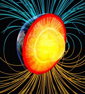
A cross-section of the earth with the field lines of the geomagnetic field . Credit: Illustration: DESY
The earth’s magnetic field has been existing for at least 3.4 billion years thanks to the low heat conduction capability of iron in the planet’s core. This is the result of the first direct measurement of the thermal conductivity of iron at pressures and temperatures corresponding to planetary core conditions. DESY scientist Zuzana Konôpková and her colleagues present their study in the scientific journal Nature. The results could resolve a recent debate about the so-called geodynamo paradox.
The geodynamo generating the earth’s magnetic field is fed on convection in the iron-rich outer core of our planet that stirs the molten, electrically conducting material like boiling water in a pot. Combined with the rotation of the earth, a dynamo effect sets in, giving rise to the geomagnetic field. “The magnetic field shields us from harmful high-energy particles from space, the so-called cosmic radiation, and its existence is one of the things that make our planet habitable,” explains Konôpková.
The strength of the convection in the outer core depends on the heat transferred from the core to the earth’s mantle and on the thermal conductivity of iron in the outer core. If a lot of heat is transferred via conduction, there is not much energy left to drive convection – and with it the earths’s dynamo. Low thermal conductivity implies stronger convection, making the geodynamo more likely to operate. “We measured the thermal conductivity of iron because we wanted to know what the energy budget of the core is to drive the dynamo,” says Konôpková. “Generation and maintenance of our planet’s magnetic field strongly depend on the thermal dynamics of the core.”
Measurements of thermal conductivity at relevant conditions proved to be difficult in the past. Recent theoretical calculations postulated a quite high thermal conductivity of up to 150 Watts per meter per Kelvin (150 W/m/K) of iron in the earth’s core. Such a high thermal conductivity would reduce the chances of the geodynamo starting up.
According to numerical models, a high thermal conductivity would have allowed the geodynamo effect to be supported only rather recently in the earth’s history, about one billion years ago or so. However, the existence of the geomagnetic field can be traced back at least 3.4 billion years. This geodynamo paradox has puzzled scientists. “There’s been a fierce debate among geophysicists because with such a large thermal conductivity, it becomes hard to explain the history of the geomagnetic field which is recorded in ancient rocks”, says Konôpková.
The physicists used a specially designed pressure cell that allows to compress samples between two diamond anvils and to heat them simultaneously with infrared lasers, shining right through the diamonds. Konôpková teamed up with Stewart McWilliams and Natalia Gómez-Pérez from the University of Edinburgh and Alexander Goncharov from the Carnegie Institution in Washington DC to measure the thermal conductivity of iron at high pressure and high temperature conditions in Goncharov’s lab.
“We compressed a thin foil of iron in the diamond anvil cell to up to 130 Giga-Pascals, which is more than a million times the atmospheric pressure and corresponds to approximately the pressure at the earth’s core-mantle boundary,” explains Konôpková. “Simultaneously we heated up the foil to up to 2700 degrees Celsius with two continuous infrared laser beams, shining through the diamonds. Finally, we used a third laser to send a low power pulse to one side of the foil to create a thermal perturbation and measured the temperature evolution from both sides of the foil with an optical streak camera.” This way the scientists could watch the heat pulse travelling through the iron.
These measurements were conducted at several pressures and temperatures to cover different conditions of planetary interiors and to obtain a systematic investigation of the thermal conductivity as a function of pressure and temperature. “Our results strongly contradict the theoretical calculations,” reports Konôpková. “We found very low values of thermal conductivity, about 18 to 44 Watts per meter per Kelvin, which can resolve the paradox and make the geodynamo operable since the early ages of the earth.”
Reference
Direct measurement of thermal conductivity in solid iron at planetary core conditions; Zuzana Konôpková, R. Stewart McWilliams, Natalia Gómez-Pérez, Alexander F. Goncharov
Nature, 2016; DOI: 10.1038/nature18009
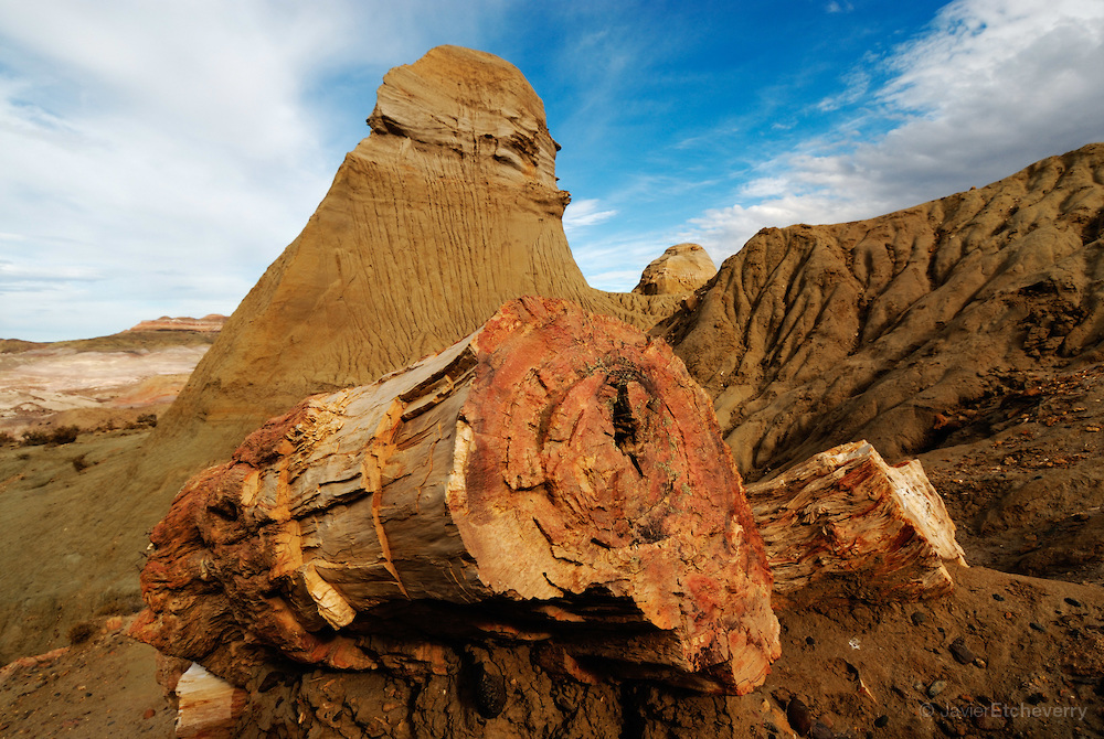
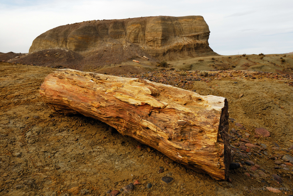
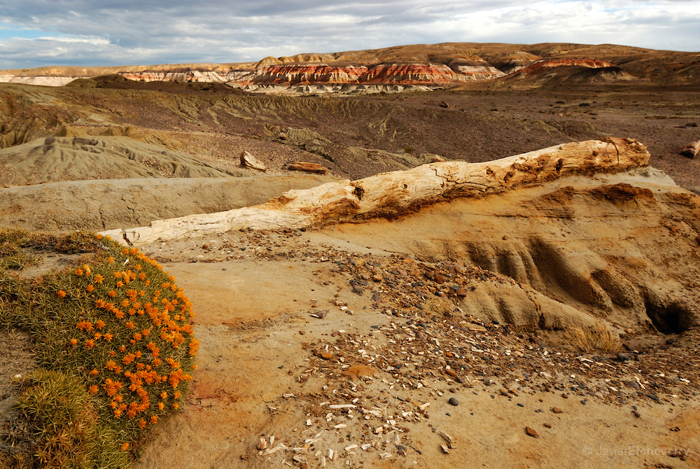
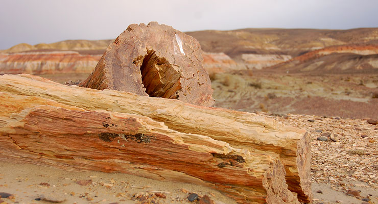
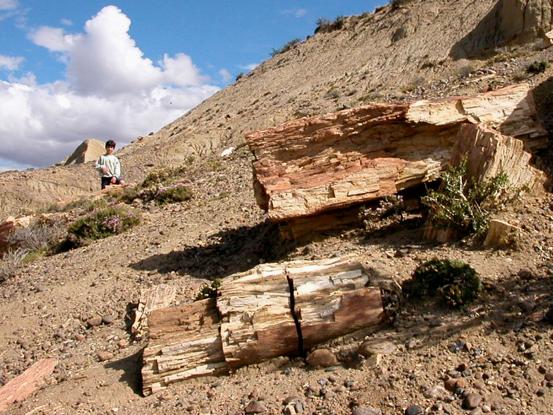
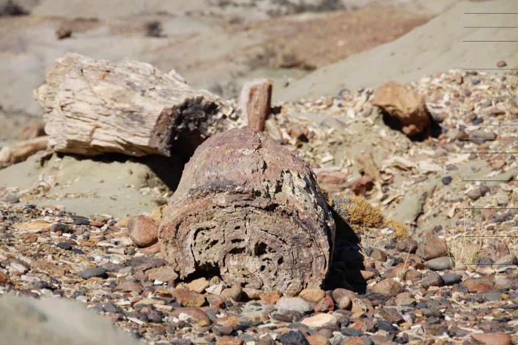
It is located just 30 km away to the South of Sarmiento, Argentina. This provincial natural monument is a forest from the Cenozoic Era. That means it is approximately 65 million years old.
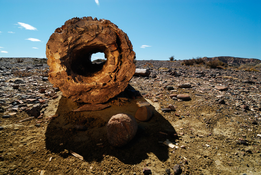
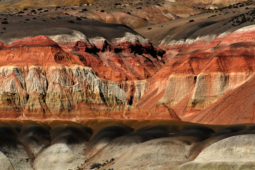
These petrified trees, witnesses of Prehistory, make up an indescribable beauty given by the hardness of the rock, the color of the different geologic strata and the heavy silence of respect for nature.
Its petrified logs are part of the result of the effect of millions of years on the wood. At the beginning of the Tertiary Era, the Andes Mountain Range rose and thus, prevented the humidity from the Pacific from getting through. At the same time, eruptions were produced and the ash deposits spread around giving way to a slow process of transformation of these logs into stone.
There are plenty of logs in the volcanic sediments of its soil. Some of them have a significant size and it has been established that they were originated in the Lower Tertiary Period (Paleocene).
The tiny grains of pollen of these sediments were studied in order to reconstruct the kind of vegetation dominating the area with extreme detail. The plants used to belong to a temperate to tropical warm kind of weather with significant humidity.
Photo
Sarmiento Petrified Forest
1 of 8
"Petrified Forest ""José Ormachea"", Sarmiento, Province of Chubut, Patagonia, Argentina, South America"
"Petrified Forest ""José Ormachea"", Sarmiento, Province of Chubut, Patagonia, Argentina, South America"
"Petrified Forest ""José Ormachea"", Sarmiento, Province of Chubut, Patagonia, Argentina, South America"
"Petrified Forest ""José Ormachea"", Sarmiento, Province of Chubut, Patagonia, Argentina, South America"
"Petrified Forest ""José Ormachea"", Sarmiento, Province of Chubut, Patagonia, Argentina, South America"
Map
Note: The above post is reprinted from materials provided by InterPatagonia.
Artist interpretation shows 190-million-year-old nests, eggs, hatchlings and adults of the prosauropod dinosaur Massospondylus in Golden Gate Highlands National Park, South Africa Credit: Julius Csotonyi
Can a crocodile’s smile reveal whether dinosaurs had lips? What if lips and gums hid most of dinosaur’s teeth?
New findings from University of Toronto vertebrate palaeontologist Robert Reisz challenge the idea of what therapods might have looked like when dinosaurs roamed the earth.
His research was presented last month at a conference at U of T Mississauga.
“When we see dinosaurs in popular culture, such as in the movie Jurassic Park, we see them depicted with big teeth sticking out of their mouths,” Reisz says. Large dinosaurs, such as Tyrannosaurus rex, bare a ferocious grin, while smaller creatures such as velociraptors are shown with scaly lips covering their teeth.
The U of T Mississauga expert was curious about which version might be most accurate. “We have very little information about dinosaurs’ soft tissue,” he says.
For clues about how therapods might have appeared, he looked to modern-day reptilian predators like crocodiles and monitor lizards. According to Reisz, lipless crocodiles have exposed teeth, much like a Jurassic Park predator, while monitor lizards conceal teeth behind scaly lips that are similar to the movie version of velociraptors.
Lips help to protect teeth, in part by helping to enclose them in a moist environment where they won’t dry out, Reisz says. Crocodiles, which spend their time submerged in water, don’t need lips for protection. “Their teeth are kept hydrated by an aquatic environment,” Reisz says.
Reptiles with lips, such as monitor lizards, typically live on land (much like their movie counterparts) where their teeth require different protection. From this, Reisz concludes that dinosaur teeth would likely have been covered by scaly lips.
“It’s also important to remember that teeth would have been partially covered by gums. If we look at where the enamel stops, we can see that a substantial portion of the teeth would be hidden in the gums. The teeth would have appeared much smaller on a living animal.
“In popular culture, we imagine dinosaurs as more ferocious-looking, but that is not the case.”
Reisz presented his findings on May 20 at the annual meeting of the Canadian Society of Vertebrate Palaeontolgy at UTM.
“Canada has some very significant locations for understanding vertebrate evolution, ranging from the late Cretaceous in Alberta to the Pleistocene in the Arctic and the early stages of terrestrial vertebrate evolution in the Atlantic region,” says Reisz, who helped to organized the conference.
“There are about 1,000 people worldwide who study vertebrate fossils. It’s important to come together and exchange ideas and unite a community that is so widespread geographically.”
University of Wyoming researchers Davin Bagdonas and Carol Frost make observations on Lankin Dome, part of the Wyoming batholith, in central Wyoming’s Granite Mountains. Credit: Myron Allen
Geophysical monitoring of the ground above active supervolcanoes shows that it rises and falls as magma moves beneath the surface of the Earth. Silica-rich magmas like those in the Yellowstone region and along the western margin of North and South America can erupt violently and explosively, throwing vast quantities of ash into the air, followed by slower flows of glassy, viscous magma.
But what do the subterranean magma chambers look like, and where does the magma originate? Those questions can’t be answered directly at modern, active volcanoes.
Instead, a new National Science Foundation (NSF)-funded study by University of Wyoming researchers suggests that scientists can go back into the past to study the solidified magma chambers where erosion has removed the overlying rock, exposing granite underpinnings. The study and its findings are outlined in a paper published in the June issue of American Mineralogist, the journal of the Mineralogical Society of America.
“Every geology student is taught that the present is the key to the past,” says Carol Frost, director of the NSF’s Division of Earth Sciences, on leave from UW, where she is a professor in the Department of Geology and Geophysics. “In this study, we used the record from past to understand what is happening in modern magma chambers.”
One such large granite body, the 2.62 billion-year-old Wyoming batholith, extends more than 125 miles across central Wyoming. UW master’s degree student Davin Bagdonas traversed the Granite, Shirley and Laramie mountains to examine the body, finding remarkable uniformity, with similar biotite granite throughout.
“It was monotonous,” says Bagdonas, who worked on the project with Frost. “Only minor variations were observed in granite near the roof and margins of the intrusion.”
This homogeneity indicates that the crystallizing magma was generally well-mixed. However, more subtle isotopic variations across the batholith show that the magma formed by melting of multiple rock sources that rose through multiple conduits, and that homogenization was incomplete.
Studies of the products of supervolcanoes and their possible batholithic counterparts at depth are a vibrant, controversial area of research, says Brad Singer, professor in the Department of Geoscience at the University of Wisconsin-Madison. He says the research by Frost and her colleagues offers “a novel perspective gleaned from the ancient Wyoming batholith, suggesting that it is the frozen portion of a vast magma system that could have fed supervolcanoes like those which erupted in northern Chile-southern Bolivia during the last 10 million years.
“The possibility of such a connection, while intriguing, does raise questions. The high silica and potassium contents of the Wyoming granites differ from the bulk magma compositions erupted by these huge Andean supervolcanos. This might mean that the Wyoming batholith records the complete solidification of potentially explosive magma at depth, without the eruption of much high-silica rhyolite,” Singer says. “Notwithstanding, this paper will certainly provoke a deeper look into how ancient Archean granites can be used to leverage understanding of the ‘volcanic-plutonic connection’ at supervolcanoes.”
Large bodies composed solely of biotite granite are more common in the Neoarchean eon (2.8 billion-2.5 billion years ago) than in younger terrains. The reason may relate to higher radioactive heat production in the past, which provided the power to drive extensive granite formation, the UW researchers say.
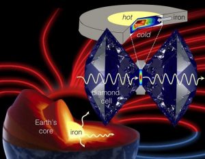
This is an illustration of how the diamond anvil cell is used to mimic and study planetary core conditions. Credit: Stewart McWilliams
Earth’s magnetic field shields us from deadly cosmic radiation, and without it, life as we know it could not exist here. The motion of liquid iron in the planet’s outer core, a phenomenon called a “geodynamo,” generates the field. But how it was first created and then sustained throughout Earth’s history has remained a mystery to scientists. New work published in Nature from a team led by Carnegie’s Alexander Goncharov sheds light on the history of this incredibly important geologic occurrence.
Our planet accreted from rocky material that surrounded our Sun in its youth, and over time the most-dense stuff, iron, sank inward, creating the layers that we know exist today–core, mantle, and crust. Currently, the inner core is solid iron, with some other materials that were dragged along down during this layering process. The outer core is a liquid iron alloy, and its motion gives rise to the magnetic field.
A better understanding of how heat is conducted by the solid of the inner core and the liquid in the outer core is needed to piece together the processes by which our planet, and our magnetic field, evolved–and, even more importantly, the energy that sustains a continuous magnetic field. But these materials obviously exist under very extreme conditions, both very high temperatures and very intense pressures. This means that their behavior isn’t going to be the same as it is on the surface.
“We sensed a pressing need for direct thermal conductivity measurements of core materials under conditions relevant to the core,” Goncharov said. “Because, of course, it is impossible for us to reach anywhere close to Earth’s core and take samples for ourselves.”
The team used a tool called a laser-heated diamond anvil cell to mimic planetary core conditions and study how iron conducts heat under them. The diamond anvil cell squeezes tiny samples of material in between two diamonds, creating the extreme pressures of the deep Earth in the lab. The laser heats the materials to the necessary core temperatures.
Using this kind of lab-based mimicry, the team was able to look at samples of iron across temperatures and pressures that would be found inside planets ranging in size from Mercury to Earth–345,000 to 1.3 million times normal atmospheric pressure and 2,400 to 4,900 degrees Fahrenheit–and study how they propagate heat.
They found that the ability of these iron samples to transmit heat matched with the lower end of previous estimates of thermal conductivity in Earth’s core–between 18 and 44 watts per meter per kelvin, in the units scientists use to measure such things. This translates to predictions that the energy necessary to sustain the geodynamo has been available since very early in the history of Earth.
“In order to better understand core heat conductivity, we will next need to tackle how the non-iron materials that went along for the ride when iron sunk to the core affect these thermal processes inside of our planet,” Goncharov added.
Reference:
Zuzana Konôpková, R. Stewart McWilliams, Natalia Gómez-Pérez, Alexander F. Goncharov. Direct measurement of thermal conductivity in solid iron at planetary core conditions. Nature, 2016; 534 (7605): 99 DOI: 10.1038/nature18009
Photo captures one of the California landslide sites studied by the UO’s Georgie Bennett and Joshua Roering. The research team they led found that California’s unprecedented drought is reflected in the drying of landslide formations and dramatic reductions in their movement. Credit: Photo courtesy of Georgie Bennett
Merged data from on-the-ground measurements, aerial photography, satellite imagery and satellite-radar imaging have unveiled an unexpected geological consequence of northern California’s ongoing drought.
Initially, University of Oregon scientists were perplexed by new satellite data that indicated that trees and rocks atop 98 slow-moving landslides in northern California’s Eel River Basin were no longer flowing at historical rates seen between 1944 and the turn of the century. Many of the formations, they could see, had barely moved in the last three years.
“We realized that this slowing down of the landslides was a massive signature of California’s drought,” said Joshua Roering, a professor in the UO Department of Geological Sciences. “Finding this was an accident. We didn’t set out to connect our research to climate. We discovered this by being frustrated by the data.”
The research, led by Roering’s postdoctoral researcher Georgie L. Bennett, is detailed in a paper accepted for publication in the journal Geophysical Research Letters. The findings, she said, are important to scientists monitoring landslides worldwide, including at similar sites she has visited in Italy.
Many Eel River Basin landslides have been slowly moving for thousands of years. The new study shows that the landslides, based on the 10 most-scrutinized landslides, slowed by half twice between 2009 and 2015, a period when the region experienced unprecedented drought.
Rates of historical movement vary by the size and depth of individual formations, Roering said, adding that, in general, the landslides had averaged “a few feet” annually. Small landslides are more sensitive to seasonal periods of rainfall and drought, while larger landslides more likely average out impacts from climate variability, the researchers found.
“Landslides move highways and make things really difficult for engineers all over the western U.S., and all over the world,” Roering said.
Understanding the interior plumbing of landslides, especially how moisture affects “the conveyor belt” that keeps them moving along the surface is vital to maintaining safety and for projecting conditions that may indicate a catastrophic collapse that could dam a river or destroy a highway, he said.
“The landslide outflows we studied are typical in many places in the world,” said Bennett, now a postdoctoral research associate with the U.S. Forest Service and Colorado State University. “This paper is important to helping understand how landslides respond to rainfall, and it provides data that should eventually help in terms of forecasting how landslides will respond to climate change. Smaller outflows are more sensitive to increasing or declining amounts of precipitation.”
The study area covered an 86-square-mile stretch along the 200-mile-long river, which meanders through the coastal mountain range from just north of California’s wine country to near Fortuna, where it meets the Pacific Ocean.
Data collection on such a scale had not been done before, Roering said. “The difference here is the amount of data we looked at,” he said. “People have been putting equipment on landslides and watching them for years — long before GPS and lasers. We were able to do this on a massive scale. This was a systematic look at the whole landscape — what it’s doing — not just of one feature.”
Researchers found that the rocks and soil have dried substantially, based on groundwater data gathered at one of the locations. The current lack of moisture, Roering said, means there is no longer enough lubrication to allow for movement.
This summer, his team, in collaboration with a team led by UO seismologist Amanda Thomas, will place 80 small seismometers in various locations on one of the landslides. The project aims to locate the underlying water table.
“A question now is how much water will it take, and how long will it take to get water down the depths at the base of these sliding surfaces to reduce the friction and get them to start moving again,” Roering said. “The site we will be instrumenting should help us better understand the structure and plumbing of landslides.”
Data merged in the research came from manual measurements of movement based on tracking trees as they surfed on the surface of earthflows between aerial photographs from 1944 to 2006 and from automatic measurements obtained through satellite pixel tracking from high-resolution imagery spanning 2009-2015. The satellite tracking was validated using the remote sensing technology interferometric synthetic aperture radar (InSAR).
Bennett, who soon will join the faculty at the University of East Anglia in England, compared the data on landslide movement from 1944 onward with an index of drought known as the Palmer Drought Severity Index.
Reference:
Joshua Roering et al. Historic drought puts the brakes on earthflows in Northern California Authors. Geophysical Research Letters, June 2016 DOI: 10.1002/2016GL068378
Allen Bondurant, U. Alaska Fairbanks, measures the soil depth to permafrost along a thermokarst lake shore in northern Alaska. Credit: USGS photo, Benjamin Jones, Nov. 2015.
In comparison to the lower 48 states, Alaskan forests, wetlands and permafrost contain larger stores of carbon, according to the first-of-its-kind assessment recently completed by the U.S. Geological Survey, the U.S. Forest Service and the University of Alaska at Fairbanks.
“This benchmark assessment establishes significant baseline information to better understand carbon dynamics in Alaskan ecosystems,” said Interior’s Deputy Secretary Mike Connor. “It provides the latest example of how Interior is applying science to our nation’s most complex resource management challenges. Nowhere is this more critical than in Alaska with its vast and diverse geography and its heightened vulnerability to climate change.”
Alaska lands make up approximately 18 percent of the nation in total area, but they contain approximately 53 percent of the carbon stock.
“Carbon stored in high latitude ecosystems is considered more vulnerable than carbon sequestered in ecosystems in the temperate zone,” said Virginia Burkett, USGS Associate Director for Climate and Land Use Change, “because average temperatures are projected to increase faster in the boreal and arctic regions during the remainder of the century.”
“This new assessment specifically reveals how soil carbon losses in Alaska are amplified by wildfires, which have increased in size and frequency with the warming Arctic climate,” Burkett noted.
Biological carbon storage — also known as carbon sequestration — is the process by which carbon dioxide (CO2) is removed from the atmosphere and stored as carbon in vegetation, soils and sediment. The USGS inventory estimates the ability of different ecosystems to store carbon.
“The cold temperatures of Alaska have led over time to the storage of vast quantities of soil and biomass carbon,” said A. David McGuire, USGS scientist and professor of land ecology at the University of Alaska Fairbanks. “A major concern for this region is how interactions among warming temperatures, permafrost thaw, more frequent wildfires, and changes in stream flow will affect carbon storage and greenhouse gas exchange.”
Presently, Alaska’s varied ecosystems act as a moderate carbon sink overall, absorbing about 3.7 million metric tons per year from the atmosphere. Even with increased permafrost thawing and more frequent and intense wildfires, future climate models show the ability of Alaska’s ecosystems to store carbon is projected to increase during the remainder of the century. This increased ability to sequester carbon is expected to occur due to increased vegetation growth prompted by longer growing seasons and other more favorable conditions. The increased vegetation growth more than counteracts increased carbon emissions from wildfires, a finding that may appear somewhat surprising.
The assessment indicates climate change will affect different ecosystems in Alaska in different ways, weakening the boreal forest as well as boreal and arctic wetlands’ ability to sequester carbon while strengthening sequestration in Alaska’s southeast forest region. Most of the total Alaska carbon stock — over 91 percent (estimated to range between 37 and 76.9 billion metric tons) — resides in soils and permafrost. From one-third to two-thirds of the state is underlain by near-surface permafrost.
Although wildfire activity varies widely from year to year, an overall upward trend in the incidence and size of wildfires is projected to increase during the remainder of the century with the boreal region of the state to be most severely affected, diminishing its capacity as a carbon sink.
A separate study conducted as part of the assessment shows that the permafrost extent could shrink by up to 25 percent by 2100, which could potentially lead to consequences such as altering landscapes, hydrology, biomes, and fire resiliency.
The assessment estimated methane emissions for wetlands in the boreal and arctic regions, indicating that the state’s wetlands are a significant source for greenhouse gas forcing potential in both the near and long-term future.
On the other hand, southeast Alaska is a productive forest region that serves as a carbon sink. The assessment estimates that the productivity of this region would increase under a scenario of climate change and forest management by 8 to 27 percent.
The assessment further projected that a substantial proportion of the spruce forests of the boreal region could be gradually replaced by birch and aspen forests. This would mean shifting habitats for wildlife and migratory birds.
The Alaska investigation constitutes the latest chapter of a nationwide study that Congress mandated for the Department of the Interior in 2007 under the Energy Independence and Security Act. Regional biologic carbon sequestration assessments for the 48 contiguous states have been published previously. Historically, national inventory assessments about carbon stock and greenhouse gas levels have not included Alaska because of its sheer size, relative lack of transportation infrastructure, and low density of field data. This extensive assessment of Alaska’s land carbon stocks is the first such study for the state and fills an important knowledge gap about carbon and greenhouse gas emissions.
“We continue to refine our knowledge of land carbon dynamics,” Burkett observed. “It is absolutely vital that we pursue a field-based understanding of the carbon cycle of the Earth in various settings so we can better understand both the natural and the human-influenced mechanisms of climate change. This assessment was based on the best available data from field surveys, remote sensing, authoritative maps, and model simulations.”
The Alaska assessment results help identify additional scientific investigations that will contribute to refining the outlook for climate change in Alaska in relation to land management actions. Two examples of needed further scientific inquiry are (1) the feedback mechanisms of a changing climate that interact with carbon pools found in the boreal and arctic regions and (2) an assessment of the consequences of climate change to wildlife, to migratory birds, and to Alaska natives who depend on the timeless continuity of ecosystems.
Reference:
Zhiliang Zhu and A. David McGuire. Baseline and Projected Future Carbon Storage and Greenhouse-Gas Fluxes in Ecosystems of Alaska. USGS, 2016 https://pubs.er.usgs.gov/publication/pp1826
General Carrera Lake (Chilean side) or Lake Buenos Aires (Argentine side) is a lake located in Patagonia and shared by Argentina and Chile. Both names are internationally accepted.
The lake has a surface of 1,850 km² of which 970 km² are in the Chilean Aysén del General Carlos Ibáñez del Campo Region, and 880 km² in the Argentine Santa Cruz Province, making it the biggest lake in Chile, and the fourth largest in Argentina. In its western basin, Lake Gen. Carrera has 586 m maximum depth.
The lake is of glacial origin and is surrounded by the Andes mountain range. The lake drains to the Pacific Ocean on the west through the Baker River.
The weather in this area of Chile and Argentina is generally cold and humid. But the lake itself has a sunny microclimate, a weather pattern enjoyed by the few settlements along the lake, such as Puerto Guadal, Fachinal, Mallín Grande, Puerto Murta, Puerto Río Tranquilo, Puerto Sánchez, Puerto Ingeniero Ibáñez and Chile Chico in Chile, and Los Antiguos and Perito Moreno in Argentina.
The area near the coast of the lake was first inhabited by criollos and European immigrants between 1900 and 1925. In 1971 and 1991, eruptions of the Hudson Volcano severely affected the local economy, especially that of sheep farming.
The Argentine side of the lake is relatively easy to access, through a strip of plains that was first used by the Tehuelches, and then by explorer Francisco Moreno. The National Route 40, created in the 1920s, also makes use of it. The Chilean side of the lake has been mostly isolated, and was for years accessed through Argentina, until the creation in the 1990s of the Carretera Austral, which connected it to the rest of Chile, and permitted the expansion of tourism in the area.
A car ferry operates between Puerto Ingeniero Ibáñez and Chile Chico in the Chilean sector of the lake.
The lake is known as a trout and salmon fishing destination.
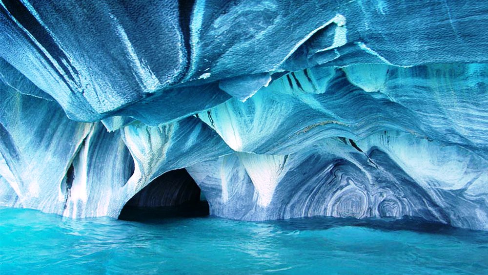
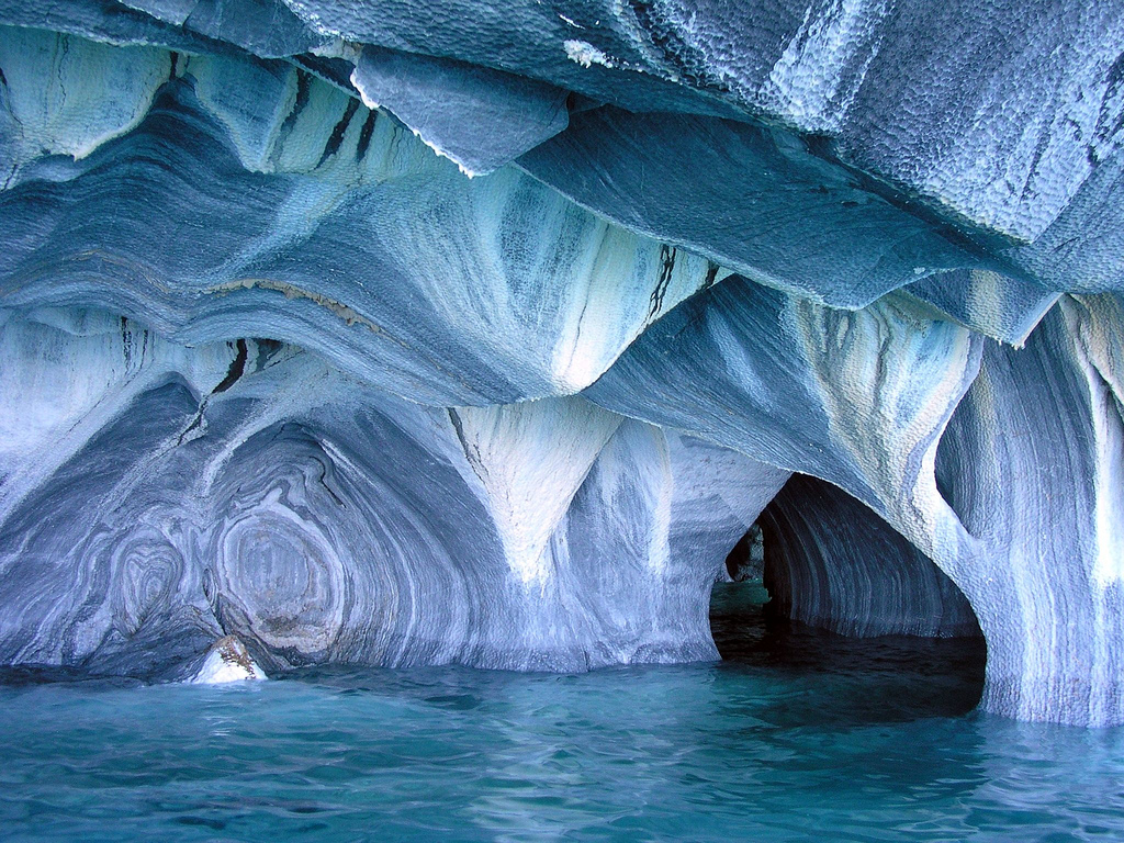
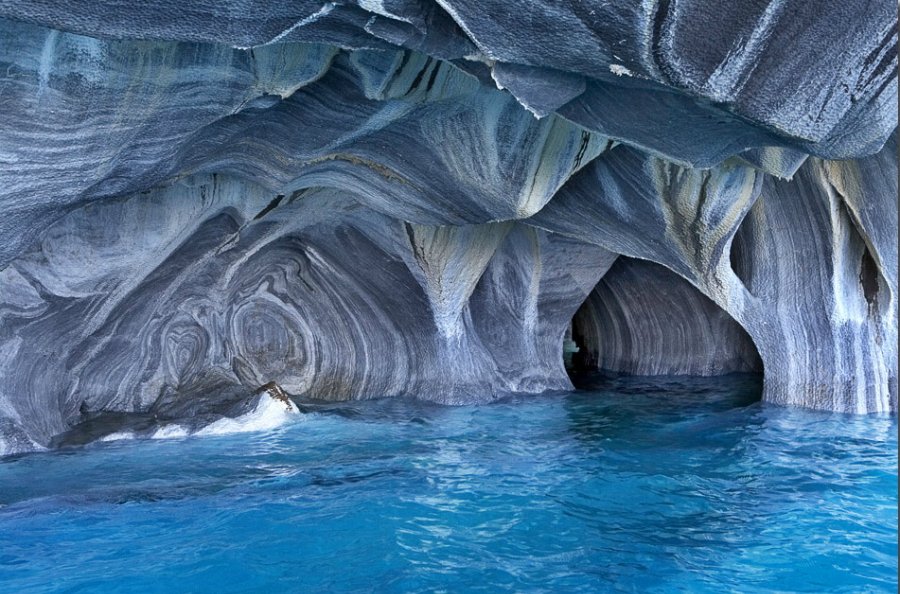
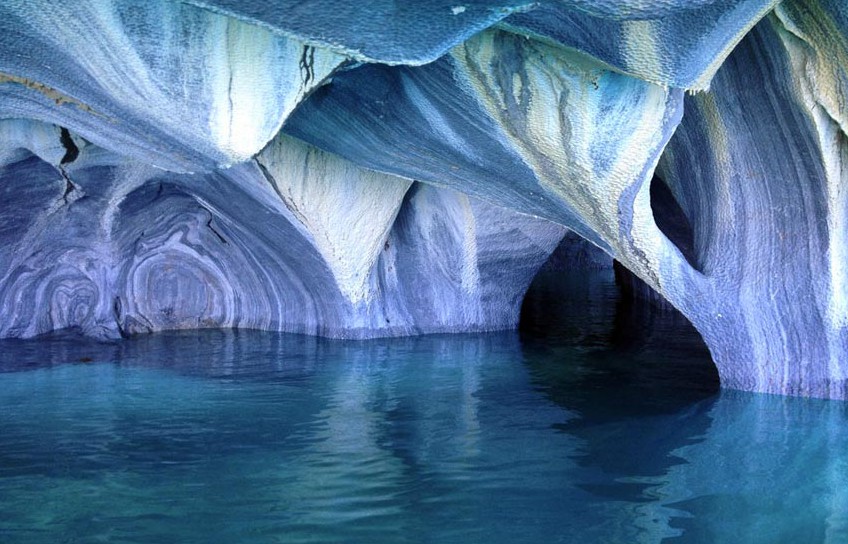
Marble Caves
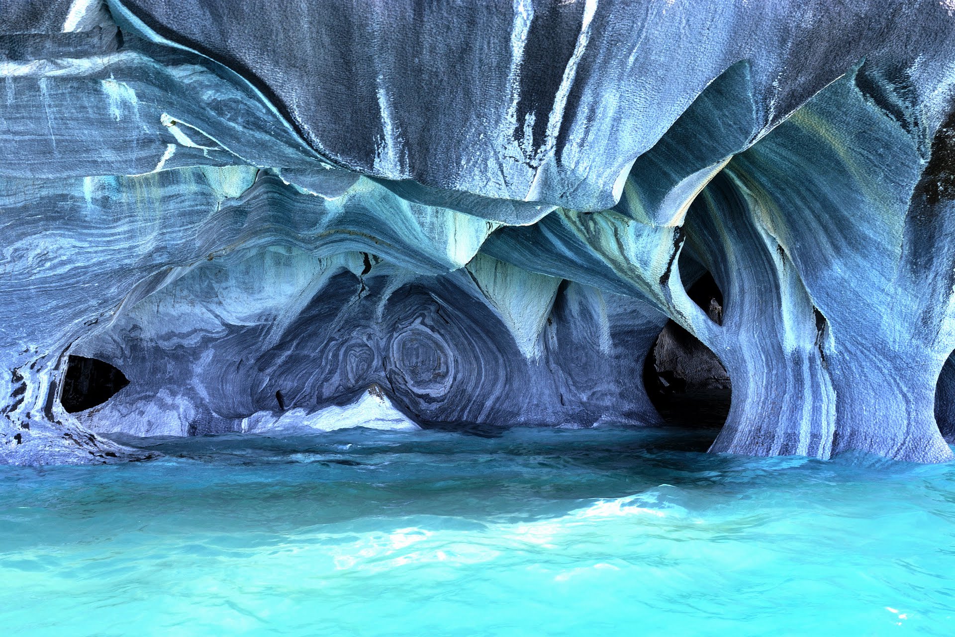
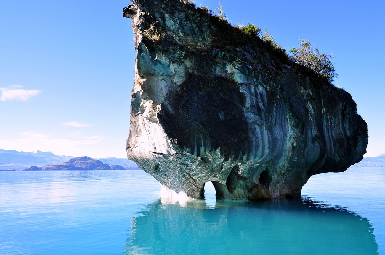
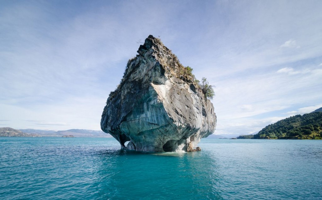
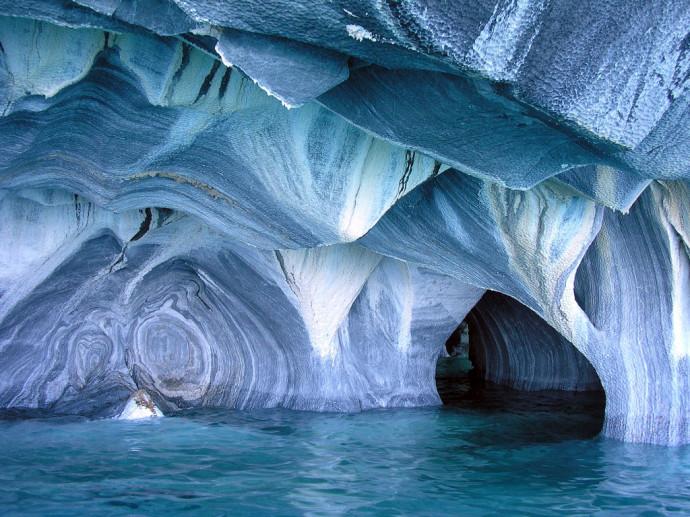
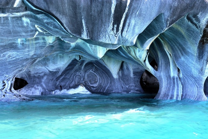
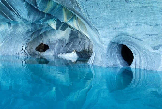
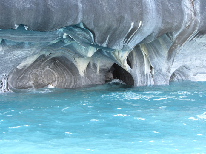
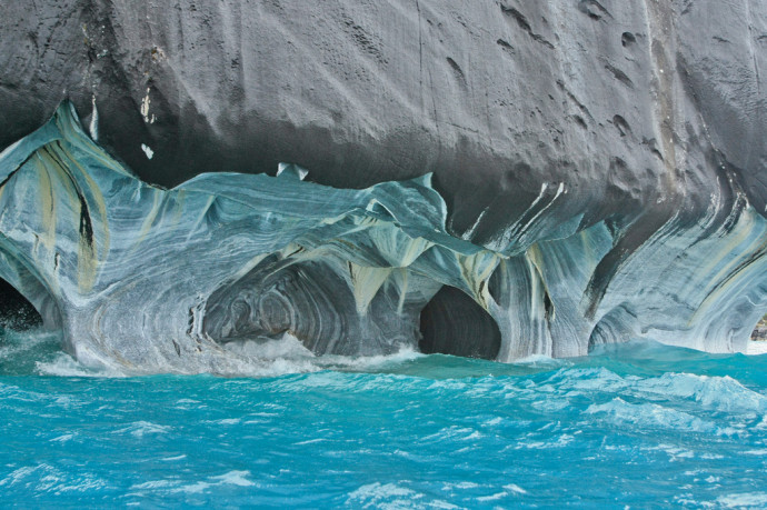
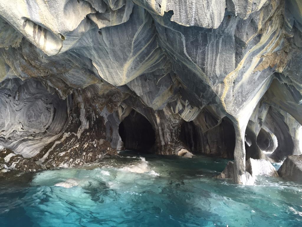
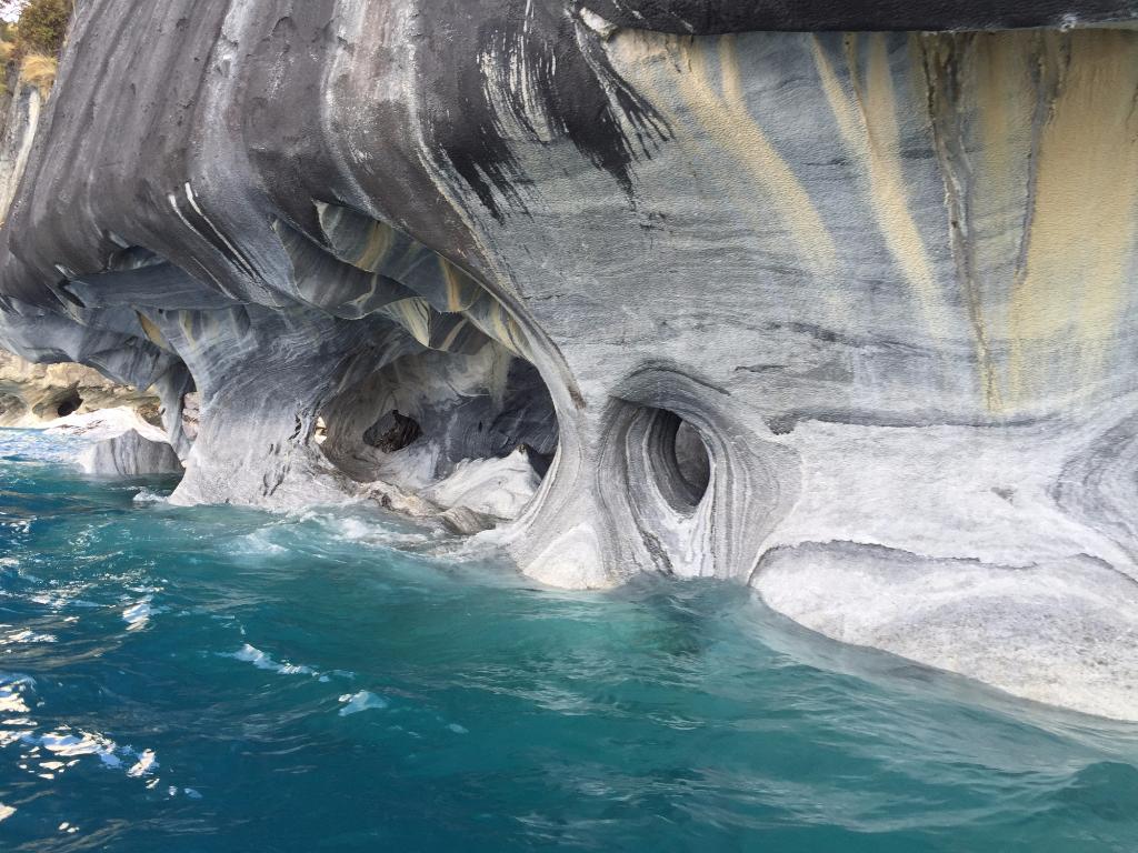
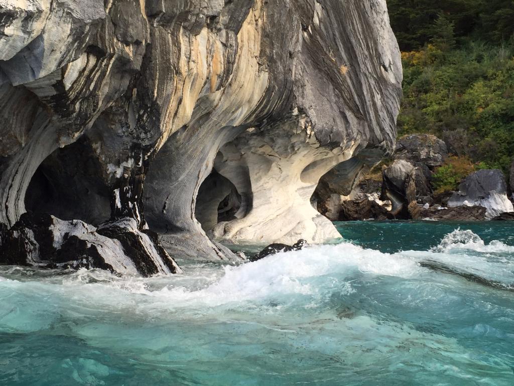
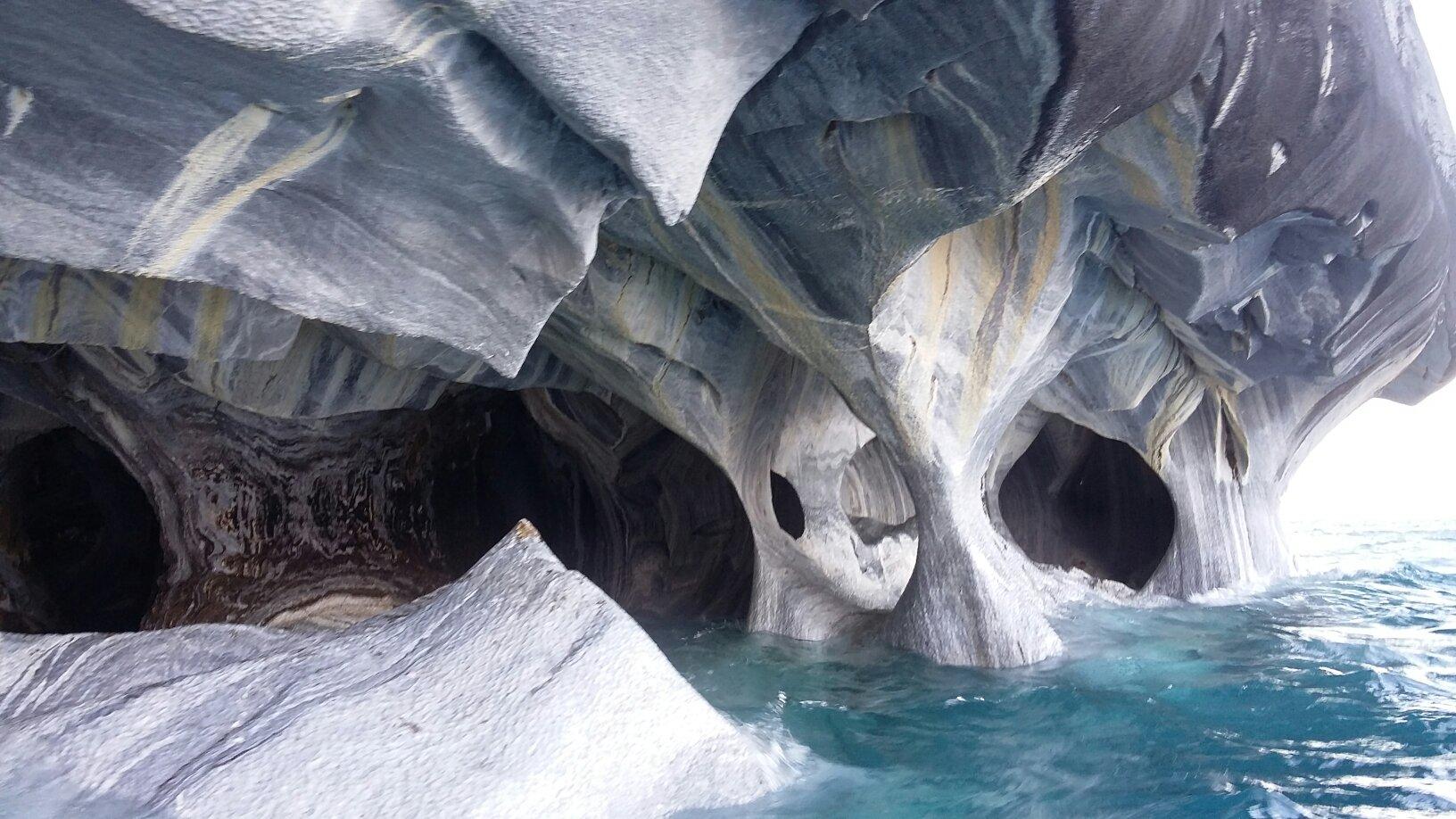
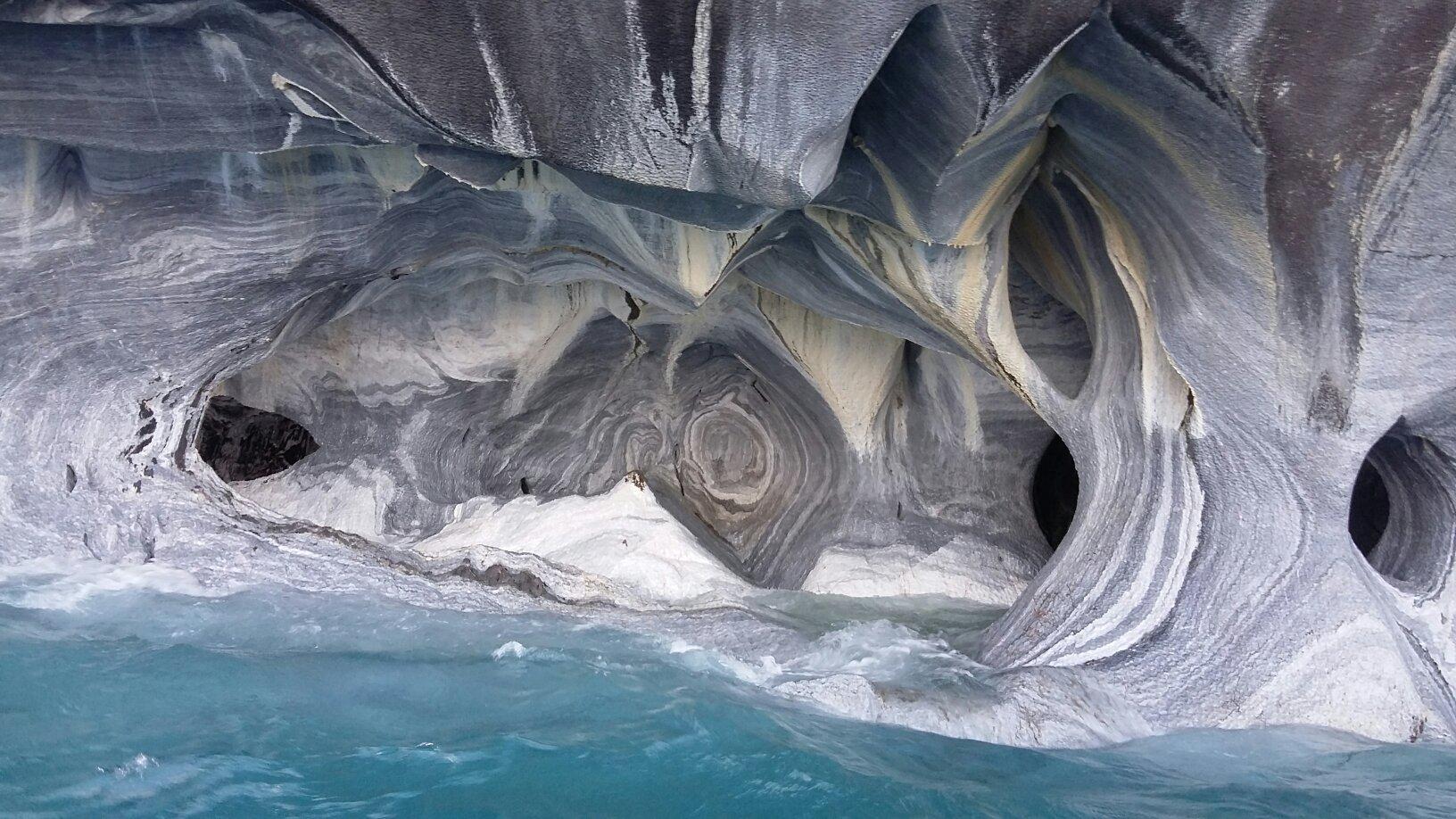
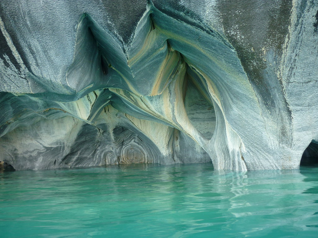
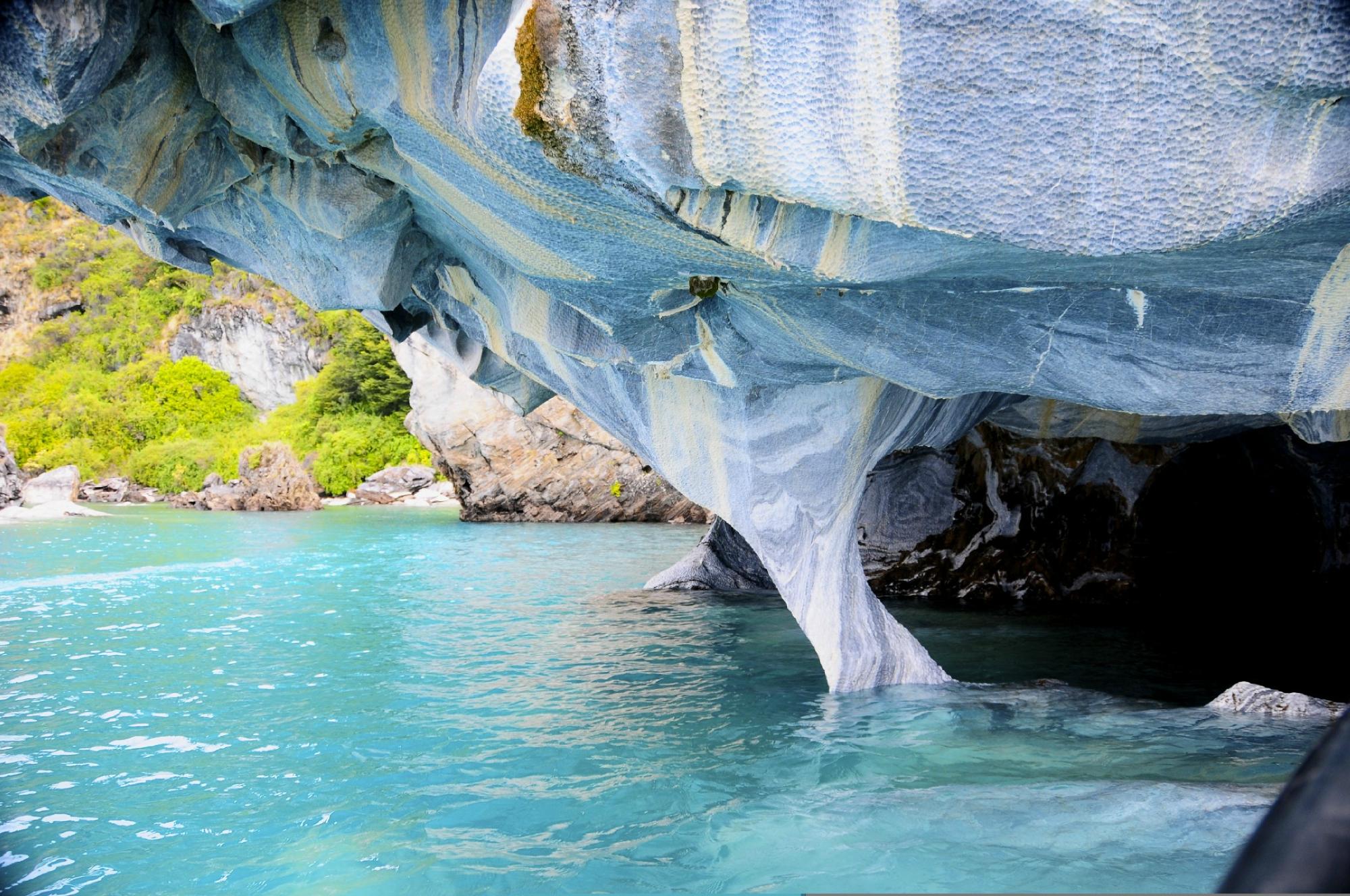
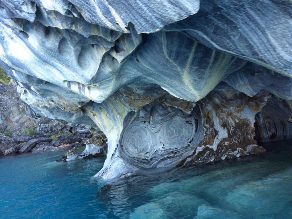
The Marble Caves is geological formation of unusual beauty. These caves have formed in a pure marble and are bathed in the deep blue water of General Carrera Lake
The Marble Chapel (Capilla de Mármol) is located in the commune of Chile Chico, in Port Calm (Puerto Tranquilo). It is formed by a massive marble peninsula, drilled by the lake, with caves at the level of the water which one enters by boat. You will be able to organize a navigation of half an hour, with one stay of equal duration that is made depending on the conditions of the weather. Sail among shining marble walls polished for the water is something truly unforgettable. These calcium carbonate formations were declared Sanctuary of the Nature (Santuario de la Naturaleza).
Blue water
The enormous General Carrera Lake is fed by rivers coming from several glaciers of Patagonian Andes.
The ice of glaciers contains small particles and, when the ice melts, many particles remain suspended in the water. This gives an unusual effect – the glacial meltwater is slightly turbid and it refracts the blue part of sunlight. Due to this the water of General Carrera Lake has a distinct blue color.
Caves, caverns, tunnels
Marble is sligthly soluble in water. Thus, when the lake reached its present level, the process of solution started at this level. The marble dissolved faster at the water surface – small seeps through the cracks in the marble made these fractures wider and waves washed away the dissolved material.
Thus, in a few thousand years time (very short time for geological processes) the interaction of the marble and blue water of lake formed a place of bewildering beauty – countless caves, mazes, columns and tunnels in the marble.
Larger, more imposing structures are Marble Cathedral and Marble Chapel. Marble Cathedral (Catedral de Mármol) is a small island at the peninsula but Marble Chapel (Capilla de Mármol) is a small marble island closer to the northern coast. One can stop his boat at one such island and take a walk… under the island, through the mazes and tunnels.
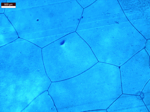
Light microscope image of as-fabricated, polycrystalline “standard” ice used for both friction and creep experiments in this study. Credit: Lamont-Doherty Earth Observatory’s Rock and Ice Mechanics Lab
Much of modern life is deeply impacted by the behavior of ice.
Now, new work from a team at Lamont-Doherty Earth Observatory at Columbia University in Palisades, New York, gives insights into what is happening inside ice. The team has developed an apparatus to meet the growing need for measuring ice as it changes in response to external forces, a process ice scientists call “deformational behaviors.” These forces occur on Earth in glacial ice as it flows due to gravity, and in space as icy satellite bodies, such as the moons of Jupiter and Saturn, respond to tidal forces from their parent bodies. These planetary icy satellites greatly intrigue scientists with their potential to hold vast oceans under the ice, and possibly, to support life.
The Lamont-Doherty team’s report on their device — called a cryogenic deformation apparatus — appears in the current issue of the Review of Scientific Instruments, from AIP Publishing.
The paper addresses three basic processes. First, the frictional process of sliding: glaciers are rivers of ice that move (“slide”) ice from centers of accumulation to oceans, a process that affects climate and water levels. The second process is anelastic behavior of an icy body, which is its ability to turn periodic mechanical energy (from tides, for instance) into heat. The third process, tidal dissipation, has recently become a focus in planetary science as a potential heat source sufficient enough to create and maintain subsurface global oceans and viscous processes affecting ice flow in which disturbances within the crystal lattice allow ice to flow like honey (over long enough time periods).
The apparatus is an adaptation of the classical biaxial friction apparatus used to study fault mechanics and earthquake generation in rocks. Another refinement of the new apparatus is its temperature control capability. It allows scientists to measure a variety of ice behaviors at conditions that are applicable to both terrestrial glaciers and icy moon surfaces. In nature, glacier temperatures are between 0 and -20 degrees Celsius (-4 degrees Fahrenheit). Ice shells of icy satellites can have warm interiors — approximately 0 degrees C — but surface temperatures as low as -200 degrees C (-330 F), like on Saturn’s moon Enceladus, though the team’s apparatus does not reach that extremely low temperature.
Temperature versatility is important because increasing evidence documents dynamic and often unpredicted behavior of ice that could affect environmental conditions — as with glaciers on earth, for example — and explain the evolution of satellites’ bodies in space, as with Jupiter’s moon Europa and Saturn’s Enceladus.
“Our design allows for both glaciological and planetary applications over a range of deformational behaviors including friction, anelastic and viscous [properties]. That range of adaptability we hope will lead to new insights about ice deformation, in particular by combining analysis of different responses and seeing how they compete at different timescales,” said Christine McCarthy, the study’s lead author.
In particular, the team hopes to extend their study of ice-on-rock friction to include more realistic interfaces, including till and, ultimately, pressurized melt water.
For their next step, the team intends to continue testing ice friction at terrestrial glacier temperatures, in particular exploring how tides affect sliding rates and stability.
For the next iteration of experiments they will dive into much deeper, colder temperatures, approximately -90 degrees C (-130 degrees F), and look at ice with small amounts of ammonia or sulfuric acid, which are second phases suggested for Enceladus and Europa, respectively.
“We’d like to see if frictional heating on faults of icy moons can explain the geysers of liquid water observed on their surfaces,” McCarthy said.
Reference:
C. McCarthy, H.M. Savage, T. Koczynski and M. Nielson. An apparatus to measure frictional, anelastic, and viscous behavior in ice at temperate and planetary conditions. Review of Scientific Instruments, 2016 DOI: 10.1063/1.4950782
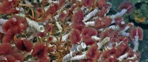
A lush community of vibrant red tube worms grows on a black smoker chimney in the ASHES hydrothermal field. The tube worms, which are hosted in white housings about the diameter of a person’s small finger, are intergrown with brown palm worms. Credit: Courtesy of University of Washington, NSF/Ocean Observatories Initiative/Canadian Scientific Submersible Facility
The hydrothermal vents and methane seeps on the ocean floor that were once thought to be geologic and biological oddities are now emerging as a major force in ocean ecosystems, marine life and global climate.
However, even as researchers learn more about their role in sustaining a healthy Earth, these habitats are being threatened by a wide range of human activities, including deep-sea mining, bottom trawling and energy harvesting, scientists say in a report published in Frontiers in Marine Science.
Researchers from Oregon State University first discovered these strange, isolated worlds on the ocean bottom 40 years ago. These habitats surprised the scientific world with reports of hot oozing gases, sulfide chimneys, bizarre tube worms and giant crabs and mussels — life forms that were later found to eat methane and toxic sulfide.
“It was immediately apparent that these hydrothermal vents were incredibly cool,” said Andrew Thurber, an assistant professor in the OSU College of Earth, Ocean and Atmospheric Sciences, and co-author on the new report.
“Since then we’ve learned that these vents and seeps are much more than just some weird fauna, unique biology and strange little ecosystems. Rather than being an anomaly, they are prevalent around the world, both in the deep ocean and shallower areas. They provide an estimated 13 percent of the energy entering the deep sea, make a wide range of marine life possible, and are major players in global climate.”
As fountains of marine life, the vents pour out gases and minerals, including sulfide, methane, hydrogen and iron — one of the limiting nutrients in the growth of plankton in large areas of the ocean. In an even more important role, the life forms in these vents and seeps consume 90 percent of the released methane and keep it from entering the atmosphere, where as a greenhouse gas it’s 25 times more potent than carbon dioxide.
“We had no idea at first how important this ecological process was to global climate,” Thurber said. “Through methane consumption, these life forms are literally saving the planet. There is more methane on the ocean floor than there are other forms of fossil fuels left in the oceans, and if it were all released it would be a doomsday climatic event.”
In reviewing the status of these marine geological structures and the life that lives around them, a group of researchers from 14 international universities and organizations have outlined what’s been learned in the past four decades and what forces threaten these ecosystems today. The synthesis was supported by the J.M. Kaplan fund.
These vents and seeps, and the marine life that lives there, create rocks and habitat, which in some settings can last tens of thousands of years. They release heat and energy, and form biological hot spots of diversity. They host extensive mussel and clam beds, mounds of shrimp and crab, create some prime fishing habitat and literally fertilize the ocean as zooplankton biomass and abundance increases. While the fluid flows from only a small section of the seafloor, the impact on the ocean is global.
Some of the microorganisms found at these sites are being explored for their potential to help degrade oil spills, or act as a biocatalytic agent for industrial scrubbing of carbon dioxide.
These systems, however, have already been damaged by human exploitation, and others are being targeted, the scientists said. Efforts are beginning to mine them for copper, zinc, lead, gold and silver. Bottom trawling is a special concern, causing physical disturbance that could interfere with seeps, affect habitat and damage other biologic linkages.
Oil, gas or hydrate exploitation may damage seeps. Whaling and logging may interfere with organic matter falling to the ocean floor, which serves as habitat or stepping stones for species reliant on chemosynthetic energy sources. Waste disposal of munitions, sewage and debris may affect seeps.
The range of ecosystem services these vents and seeps provide is just barely beginning to be understood, researchers said in their report. As many of these habitats fall outside of territorial waters, vent and seep conservation will require international collaboration and cooperation if they are going to continue to provide ecosystem benefits.
Reference:
Lisa A. Levin, Amy R. Baco, David A. Bowden, Ana Colaco, Erik E. Cordes, Marina R. Cunha, Amanda W. J. Demopoulos, Judith Gobin, Benjamin M. Grupe, Jennifer Le, Anna Metaxas, Amanda N. Netburn, Greg W. Rouse, Andrew R. Thurber, Verena Tunnicliffe, Cindy Lee Van Dover, Ann Vanreusel, Les Watling. Hydrothermal Vents and Methane Seeps: Rethinking the Sphere of Influence. Frontiers in Marine Science, 2016; 3 DOI: 10.3389/fmars.2016.00072
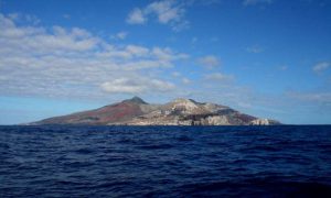
Ascension Island, located midway between Africa and Brazil will be the base of operation. A British territory, the island supports British and American air forces, communications, space agencies, and global positioning systems. Credit: Google Images
A scientist at the University of Miami (UM) Rosenstiel School of Marine and Atmospheric Science is leading an upcoming international research campaign to study a significant contributor to regional climate warming – smoke. The first-of-its-kind research experiment begins on June 1, 2016 from Ascension Island in the southeastern Atlantic Ocean. The experiment, called LASIC (Layered Atlantic Smoke Interactions with Clouds), is part of a broader international scientific collaboration led by the Atmospheric Radiation Measurement (ARM) Climate Research Facility deployment. The broad collaboration is detailed in a new article in the July Bulletin of the American Meteorological Society.
Southern Africa is the world’s largest emitter of smoke particles in the atmosphere, known as biomass-burning aerosols, from the burning of grasslands and other biomass. The project will help researchers better understand the effects of widespread biomass burning on Earth’s climate.
The study will investigate how smoke particles flowing far offshore from the African continent affect the remote and cloudy southeast Atlantic climate. Smoke, which absorbs sunlight, is a warming agent in the climate system when located above a bright surface, such as clouds. The smoke overlying the southeast Atlantic provides one of the largest aerosol-based warming of climate on the planet, since the region is also home to one of the largest low-cloud decks on the planet.
“Ascension Island is an ideal location since it is very remote and allows us to sample the smoke after it is well-aged, about which less is known,” said Paquita Zuidema, professor of atmospheric sciences at the UM Rosenstiel School and principal investigator of the research experiment. The long deployment time will allow us to characterize the marine low clouds both with and without the presence of smoke. This is ultimately valuable for understanding the Earth’s energy balance.”
By evaluating how the low clouds respond to the presence of sunlight-absorbing aerosols, scientists can better understand low cloud behavior, which is currently an uncertainty in model predictions of future climate, since no fundamental theory on low cloud processes is yet in place.
Low clouds dominate the atmosphere over the southeast Atlantic Ocean all year. Bright white cloud appears darker when viewed from above when smoke is present. The southeast Atlantic overall is brighter, not darker when smoke is present, suggesting that the clouds become thicker and more extensive when smoke is present.
Zuidema received a $365,050 seed grant from the U.S. Department of Energy to plan the study. And a $440,225 grant from NASA which further supports related aircraft investigations as part of the NASA Earth Venture Suborbital-2 ORACLES project.
NASA will complement the DOE surface-based measurements with airborne experiments during a month of each year in 2016-2018. This will allow researchers to take airborne samples of smoke particles as it ages, information that will improve satellite retrievals of this mixed smoke-cloud regime. The United Kingdom will also participate with its research aircraft, and French, Namibian, and South African scientists will collect and interpret aircraft and ground-based measurements closer to the Namibian coast.
The UM Rosenstiel School-led research team will study how smoke is transported through the atmosphere and across the Atlantic, how the aerosols change when transported, and the response of the low-lying clouds to the smoke. The information from the experiments will ultimately be used to improve global aerosol models and climate change forecasts.
Reference:
Paquita Zuidema et al. Smoke and Clouds above the Southeast Atlantic: Upcoming Field Campaigns Probe Absorbing Aerosol’s Impact on Climate, Bulletin of the American Meteorological Society (2016). DOI: 10.1175/BAMS-D-15-00082.1
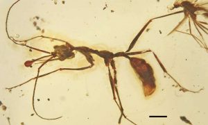
General dorsal view of holotype of new late Cretaceous worker ants Ceratomyrmex ellenbergeri. Credit: WANG Bo
Ants comprise one lineage of the triumvirate of eusocial insects and experienced their early diversification within the Cretaceous. The success of ants is generally attributed to their remarkable social behavior. Recent studies suggest that the early branching lineages of extant ants formed small colonies of either subterranean or epigeic, solitary specialist predators.
The vast majority of Cretaceous ants belong to stem-group Formicidae and comprise workers and reproductives of largely generalized morphologies, and it is difficult to draw clear conclusions about their ecology, although recent discoveries from the Cretaceous suggest relatively advanced social levels.
Remarkable exceptions to this pattern of generalized morphologies are ants with bizarre mouthparts in which both female castes have modified heads and bladelike mandibles that move along a horizontal plane rather than a vertical plane. The specific ecology of Haidomyrmecines has puzzled evolutionary biologists, who believe the mandibles apparently act as traps triggered by sensory hairs in a way distinct from that of modern trap-jaw ants.
Not all ants cooperate in social hunting, however, and some of the most effective predatory ants are solitary hunters with powerful trap jaws. Models of early ant evolution predict that the first ants were solitary specialist predators, but discoveries of Cretaceous fossils suggest group recruitment and socially advanced behavior among stem-group ants.
Dr. WANG Bo of the Nanjing Institute of Geology and Palaeontology, Chinese Academy of Sciences and his colleagues describe a new bizarre ant, Ceratomyrmex ellenbergeri, from 99 million-year-old Burmese amber that displays a prominent cephalic horn and oversized, scythelike mandibles that extend high above the head. These structures presumably functioned as a highly specialized trap for large-bodied prey. The horn results from an extreme modification of the clypeus hitherto unseen among living and extinct ants, which demonstrates the presence of an exaggerated trap-jaw morphogenesis early among stem-group ants.
Together with other Cretaceous haidomyrmecine ants, the new fossil suggests that at least some of the earliest Formicidae were solitary specialist predators. In addition, it demonstrates that soon after the advent of ant societies in the Early Cretaceous, at least one lineage, the Haidomyrmecini, became adept at prey capture, independently arriving at morphological specializations that would be lost for millions of years after their disappearance near the close of the Mesozoic. The exaggerated condition in the new fossil reveals a proficiency for carriage of large-bodied prey to the exclusion of smaller, presumably easier-to-subdue prey, and highlights a more complex and diversified suite of ecological traits for the earliest ants.
The study, entitled “Extreme morphogenesis and ecological specialization among Cretaceous basal ants,” has been published online in Current Biology.
Reference:
Vincent Perrichot et al, Extreme Morphogenesis and Ecological Specialization among Cretaceous Basal Ants, Current Biology (2016). DOI: 10.1016/j.cub.2016.03.075
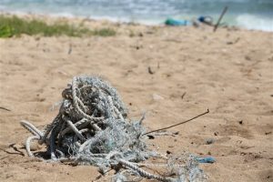
In this May 5, 2016 image provided by the state of Hawaii, ocean debris accumulates in Kahuku, Hawaii on the North Shore of Oahu. State officials say a study of the eight main Hawaiian Islands shows that ocean debris regularly accumulates around the archipelago, and that most of it is not linked to the March 2011 earthquake and tsunami in Japan. The aerial survey shows that much of the debris that accumulates on the shores of Hawaii is from fishing gear and plastics discarded locally. (Dan Dennison/Hawaii Department of Land and Natural Resources via AP)
A study of the eight main Hawaiian Islands shows that ocean debris regularly accumulates around the archipelago, and that most of it is not linked to the March 2011 earthquake and tsunami in Japan, state officials said Tuesday.
The aerial survey shows that much of the debris that accumulates on the shores of Hawaii is from items discarded carelessly across the Pacific, officials with the state Department of Land and Natural Resources said in a statement. Ocean currents can bring trash from as far away as the U.S. mainland and Asia to the shores of Hawaii.
“In order to characterize the potential ecological consequences of tsunami and other debris, it’s important to quantify it,” said Kirsten Moy, the state’s marine debris coordinator. “Understanding the types, sizes and locations of debris accumulating on Hawaiian coastlines is crucial in developing plans to streamline removal and mitigate negative impacts.”
The debris, mostly plastics but also wood, household goods, fishing gear and other items, accumulates in hot spots around the islands, mostly on the north and east shores where ocean currents deposit the trash.
The study did not examine individual pieces of debris to determine where they came from, but rather looked at the sizes and types of trash, as well as their locations, to determine what amount was produced by the 2011 tsunami and earthquake in Japan and what was not.
“This survey found a very limited amount of debris associated with the Japan tsunami,” said Suzanne Case, chairwoman of the Department of Land & Natural Resources. “Most of what was mapped is common, everyday items that someone haphazardly tossed onto the ground or directly into the water.”
The island of Niihau had the most debris in the state with nearly 8,000 pieces of debris counted. Oahu, the state’s most populated island, had the least amount of debris with just under 1,000 pieces, most of which was found on the island’s northeastern tip.
The survey was paid for by the Ministry of Environment of Japan using the Japan Tsunami Gift Fund and commissioned by the Department of Land & Natural Resources and North Pacific Marine Science Organization.
The 2011 magnitude-9.0 earthquake off the coast of northern Japan unleashed a massive tsunami. More than 19,000 people were killed, and power to a nuclear plant was cut off, triggering multiple meltdowns in the world’s second-worst nuclear disaster.
Debris from the earthquake and tsunami has been found across the Pacific, including in Hawaii where Japanese boats and other items have washed ashore.
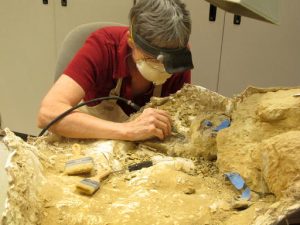
In this Saturday, May 21, 2016 photo, Anne Teppo works on a dinosaur fossil in the Museum of the Rockies in Bozeman, Mont. The museum has collected approximately 35,000 specimens over the 34 years that Jack Horner has led it. Horner retires from the museum this summer as one of the most famous paleontologists in the world. (AP Photo/Matt Volz)
Jack Horner, the paleontologist who discovered the world’s first dinosaur embryos and found that dinosaurs had nests and cared for their young, is leaving the Montana museum he spent decades filling with fossils from across the globe.
Horner, 69, Is one of the best known dinosaur researchers in the world. Michael Crichton based the character Alan Grant on Horner in the 1990 book “Jurassic Park,” and Steven Spielberg brought Horner on as a technical adviser on all of the “Jurassic Park” movies—and Horner did it without a college degree and with dyslexia.
From his base at the Museum of the Rockies in Bozeman, and before that with Princeton University, Horner discovered a dozen dinosaur species, the first dinosaur eggs in the Western Hemisphere, and provided proof of the theory of their close relation to birds. He built the Museum of the Rockies from eight dinosaur specimens when he started working there 34 years ago to more than 35,000 today.
As he ponders a state of semi-retirement, he plans to turn his attention back to education by teaching a class on imagination and creative thinking at Chapman University in California.
His struggles with dyslexia caused him to flunk out of college multiple times and initially hindered his ability to raise money for research because the grant applications had to be signed by an advanced-degree holder. He still reads at a third-grade level, and claims to have written more books than he’s read.
Horner solved one funding crisis by seeking $10,000 from the Ranier Brewing Company, whose beer he and his team drank. Princeton, his employer at the time in the late 1970s, balked and gave him the money instead.
“So Ranier Brewing Company gave us 100 cases of beer for the summer,” he said in a recent interview with The Associated Press.
That summer in 1979 would result in one of his most important discoveries—dinosaur nests on what was later called Egg Mountain in Montana. He found the site less than a mile from where he had discovered the fossils of young dinosaurs a year earlier.
“That one square mile out there is the richest dinosaur site in the world,” he said.
Little was known then about juvenile dinosaurs, and with the finds, Horner’s career path was set. The money came pouring in from the National Science Foundation and from other grants. The head of the Museum of the Rockies, tired of seeing Horner take the valuable specimens out of Montana, hired him as the museum’s paleontologist.
After that, Horner led as many as nine crews in a single digging season from Montana to Mongolia, and he started building what would become one of the largest tyrannosaurus rex and triceratops collections in the world.
Horner for the last several years has been working on the chickenosaurus, or dino-chicken. His idea is to revive dormant dinosaur DNA found in chickens to give them some traits of their ancestors, such as a long tail.
Horner said work continues on that project, and he will likely set up a laboratory for it in California, but his focus is being pulled to other things, as well. He has five books in the works, including an autobiography. He said he is helping Microsoft develop an app, but declined to speak about it in any detail.
He also won’t give up dinosaur hunting. The University of Washington is planning to open its new Burke museum, and Horner has agreed to be a part-time research associate to help fill the museum up with dinosaurs.
The Museum of the Rockies is overflowing with dinosaur fossils after 34 years of Horner as its curator of paleontology. A planned expansion will allow the museum to bring its vast collection under one roof, but there won’t be any room for him to bring in anything new to work on, he said.
“I filled this place up. There’s no reason to just stay,” Horner said. “I would just be—what do you call it—resting on your laurels or something?”
The Museum of the Rockies, which is a part of Montana State University, hasn’t found a new curator yet. Members of Horner’s team who will remain in Bozeman say he will be difficult to replace, but the museum is strong enough now to stand on its own.
“We may have a lag while we get re-established with a new curator, but I don’t see us diminishing and going away,” said Jamie Jette, who worked with Horner for 18 years.
For his part, Horner is most interested in applying his approach to paleontology to the education system. He made his most famous discoveries because he was unafraid to take a hammer to a dinosaur egg when everybody else thought eggs were too precious to crack, he said.
“I made a discovery because I had a hammer,” Horner said. “That kind of thinking is basically what I made my career on.”
A gemstone or gem is a piece of mineral crystal, which, in cut and polished form, is used to make jewelry or other adornments. However, certain rocks (such as lapis lazuli) or organic materials that are not minerals (such as amber or jet), are also used for jewelry, and are therefore often considered to be gemstones as well. Most gemstones are hard, but some soft minerals are used in jewelry because of their luster or other physical properties that have aesthetic value. Rarity is another characteristic that lends value to a gemstone. Apart from jewelry, from earliest antiquity engraved gems and hardstone carvings, such as cups, were major luxury art forms. A gem maker is called a lapidary or gemcutter; a diamond worker is a diamantaire.
Types of Gemstone
Precious stones
Semi-precious gemstones
Precious Stones
Precious stones are defined as visually appealing gemstones created from rocks or minerals. Often used for jewelry and fashion accents, this term was created in the mid-1800’s to refer to four specific stones; diamonds, rubies, emeralds, and sapphires. All precious stones are translucent and are valued by the richness of their color, except for the diamond, which has a higher value based on being colorless. Their rarity, beauty, and method in which they are produced all add to the allure of a precious stone. Any accessory containing a precious stone would be deemed sophisticated and worn by someone of high class.
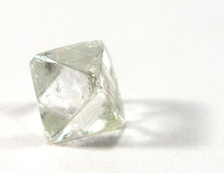
1-Diamond
Locality: Kimberley, Francis Baard District, Northern Cape Province, South Africa Dimensions: 7 mm x 6 mm x 6 mm “Courtesy of Rob Lavinsky, The Arkenstone, www.iRocks.com”
Chemical Formula: C Locality: Kimberly, republic of South Africa. India. Brazil. Ural Mountains, Russia. Murfreesboro, Arkansas, USA. Name Origin: From the Greek, adamas, meaning “invincible” or “hardest.”
In mineralogy, diamond is a metastable allotrope of carbon, where the carbon atoms are arranged in a variation of the face-centered cubic crystal structure called a diamond lattice. Diamond is less stable than graphite, but the conversion rate from diamond to graphite is negligible at standard conditions. Diamond is renowned as a material with superlative physical qualities, most of which originate from the strong covalent bonding between its atoms. In particular, diamond has the highest hardness and thermal conductivity of any bulk material. Those properties determine the major industrial application of diamond in cutting and polishing tools and the scientific applications in diamond knives and diamond anvil cells.
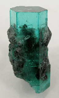
2-Emerald
Emerald with Calcite Muzo Mine, Boyaca Dept., Colombia Thumbnail, 2.9 x 1.4 x 1.2 cm “Courtesy of Rob Lavinsky, The Arkenstone, www.iRocks.com”
Color: Emerald Green to Dark Green Mohs hardness scale: 7.5 – 8 Mineral Class: Beryl Locality: Found in Columbia, Brazil, Zimbabwe, South Africa, Afghanistan, USA
Emerald is a gemstone and a variety of the mineral beryl (Be3Al2(SiO3)6) colored green by trace amounts of chromium and sometimes vanadium. Beryl has a hardness of 7.5–8 on the Mohs scale. Most emeralds are highly included, so their toughness (resistance to breakage) is classified as generally poor.
3-Ruby
Cut ruby gemstone with inclusions Credit: Humanfeather
Color: Bright red, brownish-red, purplish-red, dark red Mohs hardness scale: 9 Mineral Class: Corundum Locality: Found mainly in Burma, Thailand, Sri Lanka and Tanzania
A ruby is a pink to blood-red colored gemstone, a variety of the mineral corundum (aluminium oxide). The red color is caused mainly by the presence of the element chromium. Its name comes from ruber, Latin for red. Other varieties of gem-quality corundum are called sapphires. Ruby is considered one of the four precious stones, together with sapphire, emerald and diamond.
Prices of rubies are primarily determined by color. The brightest and most valuable “red” called blood-red or “pigeon blood”, commands a large premium over other rubies of similar quality. After color follows clarity: similar to diamonds, a clear stone will command a premium, but a ruby without any needle-like rutile inclusions may indicate that the stone has been treated. Cut and carat (weight) are also an important factor in determining the price. Ruby is the traditional birthstone for July and is usually more pink than garnet, although some rhodolite garnets have a similar pinkish hue to most rubies. The world’s most expensive ruby is the Sunrise Ruby.
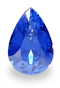
4-Sapphire
Pear-shaped blue sapphire Credit: LesFacettes
Color: Blue, Yellow, Green, White, Colorless, Pink, Orange, Brown and Purple Mohs hardness scale: 9 Mineral Class: Corundum Locality: Found mainly in Sri Lanka, Thailand, Burma, Australia, India, Brazil and Africa
Sapphire is a typically blue gemstone variety of the mineral corundum, an aluminium oxide (α-Al2O3). Trace amounts of elements such as iron, titanium, chromium, copper, or magnesium can give corundum respectively blue, yellow, purple, orange, or green color. Chromium impurities in corundum yield pink or red tint, the latter being called ruby.
Commonly, sapphires are worn in jewelry. Sapphires may be found naturally, by searching through certain sediments (due to their resistance to being eroded compared to softer stones) or rock formations. They also may be manufactured for industrial or decorative purposes in large crystal boules. Because of the remarkable hardness of sapphires – 9 on the Mohs scale (the third hardest mineral, after diamond at 10 and moissanite at 9.5) – and of aluminium oxide in general, sapphires are used in some non-ornamental applications, including infrared optical components, such as in scientific instruments; high-durability windows; wristwatch crystals and movement bearings; and very thin electronic wafers, which are used as the insulating substrates of very special-purpose solid-state electronics (especially integrated circuits and GaN-based LEDs).
Semi-precious stones
A semi-precious stone is also known as a gem or gemstone (also a jewel, a gem, a precious stone), which is a portion of mineral, which, in refined and cut form, is used to create jewelry or other embellishments. There are also organic resources or precise rocks that are not minerals (for example jet or amber) that are also used for jewelry and would also be considered to be gemstones, as well. In the West, precious stones are diamonds, sapphires, rubies and emeralds. All other stones are considered semi-precious stones. However, this is a commercial based classification and was a distinction that marketers created years ago which gives the false impression that precious stones are more valuable than semi-precious stones. For example, a Tsavorite green garnet is more valuable than a mid-quality sapphire. It’s a concept from the West that often puts misconceived notions of the truth into consumers’ minds. So contextually there is a difference between semi-precious and precious but it is mostly for show and strictly from a commercial perspective.
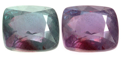
1-Alexandrite
Alexandrite Cushion, 26.75 cts. Bluish green in daylight and purple red under incandescent light, alexandrites this large are extremely rare. Credit: David Weinberg
Color: Dark to Pale Green (color is changed in different forms of lights) Mohs hardness scale: 8.5 Mineral Class: Chrysoberyl Locality: Found mainly in Russia, Sri Lanka, Brazil, Burma, Madagascar, USA
The alexandrite variety displays a color change (alexandrite effect) dependent upon the nature of ambient lighting. Alexandrite effect is the phenomenon of an observed color change from greenish to reddish with a change in source illumination. Alexandrite results from small scale replacement of aluminium by chromium ions in the crystal structure, which causes intense absorption of light over a narrow range of wavelengths in the yellow region (580 nm) of the visible light spectrum. Because human vision is more sensitive to light in the green spectrum and the red spectrum, alexandrite appears greenish in daylight where a full spectrum of visible light is present and reddish in incandescent light which emits less green and blue spectrum. This color change is independent of any change of hue with viewing direction through the crystal that would arise from pleochroism.
Alexandrite from the Ural Mountains in Russia can be green by daylight and red by incandescent light. Other varieties of alexandrite may be yellowish or pink in daylight and a columbine or raspberry red by incandescent light.
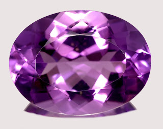
2-Amethyst
Color: Purple, Pale lavender to deep reddish purple, bluish violet Mohs hardness scale: 7 Mineral Class: Quartz Locality: Found mainly in Sri Lanka, Brazil, Burma, Canada, East Africa, India, North America, Russia, Uruguay, Madagascar and Australia
Amethyst is a violet variety of quartz often used in jewelry. The name comes from the Ancient Greek ἀ a- (“not”) and μέθυστος méthystos (“intoxicated”), a reference to the belief that the stone protected its owner from drunkenness. The ancient Greeks wore amethyst and made drinking vessels decorated with it in the belief that it would prevent intoxication. It is one of several forms of quartz. Amethyst is a semiprecious stone and is the traditional birthstone for February.
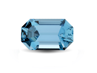
3-Aquamarine
Credit: GIA
Color: Blue, Sea-green Mohs hardness scale: 7.5 – 8 Mineral Class: Beryl Locality: Found mainly in Brazil, Madagascar, Russia, Afghanistan, India, Pakistan, Nigeria, Zambia, Mozambique and USA
Aquamarine is a blue or cyan variety of beryl. It occurs at most localities which yield ordinary beryl. The gem-gravel placer deposits of Sri Lanka contain aquamarine. Clear yellow beryl, such as that occurring in Brazil, is sometimes called aquamarine chrysolite. The deep blue version of aquamarine is called maxixe. Maxixe is commonly found in the country of Madagascar. Its color fades to white when exposed to sunlight or is subjected to heat treatment, though the color returns with irradiation.
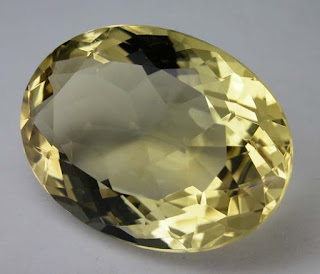
4-Citrine
Credit: Wikipedia
Color: Light Yellow, Lemon Yellow, Amber-Brown, Brilliant Orange Mohs hardness scale: 7 Mineral Class: Quartz Locality: Found mainly in South America, Brazil, Madagascar, Argentina, Russia, Scotland and Spain
Citrine, the most common reference for which is certain coloured varieties of quartz which are a medium deep shade of golden yellow. Citrine has been summarized at various times as yellow, greenish-yellow, brownish yellow or orange.
The original reference point for the citrine colour was the citron fruit. The first recorded use of citrine as a colour in English was in 1386. It was borrowed from a medieval Latin and classical Latin word with the same meaning. In late medieval and early modern English the citrine colour-name was applied in a wider variety of contexts than it is today and could be “reddish or brownish yellow; or orange; or amber (distinguished from yellow)”. In today’s English citrine as a colour is mostly confined to the contexts of (1) gemstones, including quartz, and (2) some animal and plant names. E.g., the citrine wagtail (Motacilla citreola), an Asian bird species with golden-yellow plumage.
5-Garnet
Credit: GIA
Color: Light Red, Violet, Red, White, Green, Yellow, Brown, Black Mohs hardness scale: 6.5-7.5 Mineral Class: Quartz Locality: Found mainly in Burma, Sri Lanka, South Africa, China, USA, Tanzania, Madagascar, India and Australia
Garnets are a group of silicate minerals that have been used since the Bronze Age as gemstones and abrasives.
All species of garnets possess similar physical properties and crystal forms, but differ in chemical composition. The different species are pyrope, almandine, spessartine, grossular (varieties of which are hessonite or cinnamon-stone and tsavorite), uvarovite and andradite. The garnets make up two solid solution series: pyrope-almandine-spessartine and uvarovite-grossular-andradite.
6-Grossular
Grossular is a calcium-aluminium mineral species of the garnet gemstone group with the formula Ca3Al2(SiO4)3, though the calcium may in part be replaced by ferrous iron and the aluminium by ferric iron. The name grossular is derived from the botanical name for the gooseberry, grossularia, in reference to the green garnet of this composition that is found in Siberia. Other shades include cinnamon brown (cinnamon stone variety), red, and yellow.
Grossular should not be called grossularite, grossularite was once a type of rock.
7-Pyrope
The mineral pyrope is a member of the garnet group. Pyrope is the only member of the garnet family to always display red colouration in natural samples, and it is from this characteristic that it gets its name: from the Greek for fire and eye. Despite being less common than most garnets, it is a widely used gemstone with numerous alternative names, some of which are misnomers. Chrome pyrope, and Bohemian garnet are two alternative names, the usage of the latter being discouraged by the Gemological Institute of America. Misnomers include Colorado ruby, Arizona ruby, California ruby, Rocky Mountain ruby, Elie Ruby, Bohemian carbuncle, and Cape ruby.
8-Almandine
Almandine, also known incorrectly as almandite, is a species of mineral belonging to the garnet group. The name is a corruption of alabandicus, which is the name applied by Pliny the Elder to a stone found or worked at Alabanda, a town in Caria in Asia Minor. Almandine is an iron alumina garnet, of deep red color, inclining to purple. It is frequently cut with a convex face, or en cabochon, and is then known as carbuncle. Viewed through the spectroscope in a strong light, it generally shows three characteristic absorption bands.
9-Rhodalite
Rhodolite is a varietal name for rose-pink to red mineral pyrope, a species in the garnet group. It is found in Cowee Valley, Macon County, North Carolina. The name is derived from the Greek for “rose-like”, in common with many pink mineral types (e.g. rhodochrosite, rhodonite). Rhodolite itself is not officially recognized as a mineralogical term. This coloration, and the commonly inclusion-free nature of garnet from this locality, has led to rhodolite being used as a semi-precious gemstone.
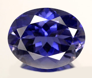
10-Iolite
Color: Violet-Blue, Deep Blue, Light Blue-Gray, Yellow-White Mohs hardness scale: 7 – 7.5 Mineral Class: Cordierite Locality: Found mainly in India, Sri Lanka, Mozambique, Zimbabwe and Brazil
The name Iolite comes from the Greek word ‘Ion’, which means ‘Violet’. Iolite is often confused with Tanzanite because of its similarity in color. Generally, Iolite is a deeper shade of violet, with hues ranging from deep blue, purple, lavendar, and gray-blue.
This gem was actually used as a navigation tool by Viking explorers. Thin pieces of Iolite were cut and used as polarizing filter lenses. Looking through the lens, they could determine the exact position of the sun and use it to guide them to the New World and back.
Iolite is relatively hard but should be protected from blows. With its attractive color and reasonable price, it may become a jewelry staple in the future.
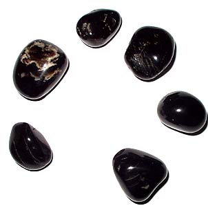
11-Onyx
Black onyx with bands of colors Credit: Wikipedia
Color: Black, White, Black with White bands, Red, Brown Mohs hardness scale: 6.5 – 7 Mineral Class: Quartz Locality: Found mainly in Madagascar, India, Brazil, United States, Pakistan and Sri Lanka
Onyx is a banded variety of the oxide mineral chalcedony. Agate and onyx are both varieties of layered chalcedony that differ only in the form of the bands: agate has curved bands and onyx has parallel bands. The colors of its bands range from white to almost every color (save some shades, such as purple or blue). Commonly, specimens of onyx contain bands of black and/or white.
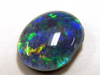
12-Opal
Color: Black, White, Gray, Yellow, Red, Orange and Colorless Mohs hardness scale: 5 – 6.5 Locality: Found mainly in Australia, Brazil, Mali, Japan, Russia, USA, Mexico
Opal is a very popular gemstone, mainly due to its wonderful variety of rich and beautiful colors. One of the extraordinary features of this gemstone is called Opalescence. Opalescence is a kind of light play that happens with certain high quality stones. Light reflects and bounces around the very small structures of the stone, giving it a wonderful aura and sometimes iridescence.
The name Opal is derived from three sources: Sanskrit ‘Upala’, Latin ‘Opalus’, and Greek ‘Opallios’. All three of these words mean the same thing – precious stone. The group of fine Opals includes quite a number of wonderful gemstones. These gemstones are differentiated on the basis of the variety, place of occurrence, and color of the main body, into Dark or Black Opal, White or Light Opal, Milk or Crystal Opal, Boulder Opal, Opal Matrix, Mexican and Fire Opal.
Opals come in many colors, including black, white, gray, yellow, colorless, orange and red. Red is considered the most popular and attractive colors that Opal comes in. There are usually two types of red colors – cherry red and fire red. Fire red is usually the most popular and possibly the most expensive due to its wonderful hue.
Australia is the major supplier of Fine Opals and almost 95 per cent of all Opals come from Australian mines. Opal is made from sand and water. It has the same chemical formula as quartz with the addition of 3 to 10 % water content. And due to this reason, opals must be protected from harsh light and heat, which could dry it out and cause cracks. Opal is relatively less hard than many other stones and must be worn with caution and care to avoid chips or other breakage. Opals come in many attractive colors, shapes and sizes and are used on many types of ornamental jewelry including rings, earring rings, brooches, charms, bracelets, etc.
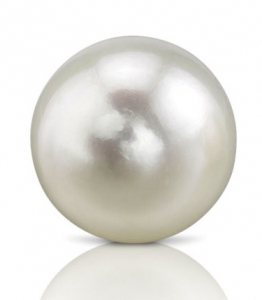
13-Pearl
Color: White, White tinted with Cream, Pink, Yellow, Green, Blue, Brown, Purple, or Black. Mohs hardness scale: 2.5 – 4.5 Locality: Found mainly in Persian Gulf, China Sea
A Pearl is an organic gem, produced when certain mollusks, primarily oysters cover a foreign object with beautiful layers of nacre. A good sized Pearl can take between five to eight years to form, which is usually the entire life of the oyster or mollusk.
There are two types of Pearls: Natural Pearls, formed inside wild oysters, practically impossible to find nowadays, and Cultured Pearls in which the production of the pearl is artificially induced. For producing cultured pearls, shell beads are placed inside an oyster and the oyster is returned to the water. When the pearls are later harvested, the oyster has covered the bead with layers of nacre. The finest Natural Pearls are fished almost exclusively from the Persian Gulf and the China Sea, while the best cultivated ones come from Japan, Korea and more recently Australia. Fine Natural Pearls are much more expensive and rare to find than Cultured Pearls.
Pearls are usually white, sometimes with a creamy or pinkish tinge, but may be tinted with yellow, green, blue, brown, purple, or black. Pearls are available in different shapes: round, semi-round, button, drop, pear, oval, baroque, and ringed. Perfectly round Pearls are the rarest and most expensive. Pearl is a rare and living substance and should be treated with great care.
14-Peridot
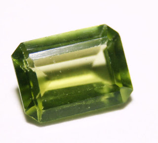
Emerald Cut Peridot ready to set in jewellery. Credit: Michelle Jo
Color: Yellow Green, Olive, Brownish Green Mohs hardness scale: 6.5 – 7 Mineral Class: Olivine Locality: Found mainly in Australia, Mexico, Sri Lanka, South Africa, Tanzania, China, Burma, Arizona, USA, Pakistan, Afghanistan
The Peridot is a very old but still very popular gemstone. It is a verity of mineral olivine. The color of most gemstones is caused by traces of other elements but the color of Peridot is an integral part of its structure. Chemically Peridot is an iron-magnesium-silicate. The intensity of the color of the stone depends upon the amount of iron contained. The beauty of Peridot is a result of extreme conditions. Peridot is formed deep within the earth under tremendous heat and pressure.
This gemstone is in fact identified by three names, Peridot, Chrysolith and Olivin. ‘Peridot’ is derived from Greek word ‘Peridona’, which mean ‘giving plenty’. The word ‘Chrysolith’ means ‘goldstone’ in Greek. It is one of the few stones that exist only in one color. The most beautiful Peridot comes from Pakistan-Afghanistan border region. It is also found in Australia, Mexico, Sri Lanka, South Africa, Tanzania, China, Burma, Arizona and USA. Peridot is used in rings, earrings, pendants, bracelets.
15-Tanzanite
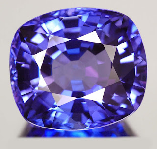
Color: Deep Blue, Ultramarine Blue, Light Violet-Blue, Purple Mohs hardness scale: 6 – 7 Mineral Class: Quartz Locality: Found in Tanzania
Tanzanite is an extraordinary and beautiful gemstone. Tanzanite is a blue variety of the gemstone zoisite discovered in 1967 at Merelani Hills in Tanzania. It is named after the East African state of Tanzania, the only place in the world where it has been found. Due to this reason, this stone is particularly highly prized.
Tanzanite is a trichroic gem which displays three layers of color. The colors dark blue, green-yellow and red-purple can be seen. Nearly all tanzanite has been heat treated to generate the beautiful violet-blue color this stone is known for.
Although Tanzanite is relatively new on the gemstone market, but has left its mark. Tanzanite is popular for its brilliance and widely distributed gemstone. But on the same time, Tanzanite is a delicate gemstone and it should always be worn carefully. Never clean tanzanite in an ultrasonic cleaner or resize or repair a Tanzanite ring set without having the gem removed because the stone could shatter in the heat of a torch.
16-Topaz
Azotic Topaz
Color: Blue, Brown, Green, Orange, Pink, Red, Yellow, White, Gold, Colorless Mohs hardness scale: 8 Mineral Class: Topaz Locality: Found mainly in Brazil, Sri Lanka, Burma, Nigeria, USA, Australia, Madagascar and Mexico
Topaz is a member of Quartz family. This beautiful gemstone most commonly found in yellow color. A Topaz turns a vivid blue when exposed to heat. Also the Topaz is said to have power of changing color when it’s near poison. The name topaz is derived from the Sanskrit word ‘Tapas’, meaning ‘Fire’.
Although Topaz is considered tough and durable gemstone but still it is not an invincible stone. It cracks and chips easily than many other gemstones, and should be treated with care.
17-Tourmaline
11.21-carat Bicolor Tourmaline Credit: GIA
Color: Black, Red, Pink, Blue, Green, Grey and Yellow Mohs hardness scale: 7 – 7.5 Mineral Class: Quartzite Locality: Found mainly in Brazil, Sri Lanka, South Africa, Nigeria, Zimbabwe, Kenya, Tanzania, Mozambique, Madagascar, Pakistan, Afghanistan, USA
Tourmalines are gemstones with deep brilliance and incomparable variety of colors. These Gemstones are mixed crystals of aluminium boron silicate with a complex and changing composition.
The name tourmaline comes from the Singhalese words ‘tura mali’, means something like ‘stone with mixed colors’. Tourmalines with different colors have different names. For example, a tourmaline of an intense red is known as a ‘rubellite’, but if it changes the color on change in the light source then the stone is called pink or shocking pink tourmaline. Stones with two colors are known as bicolored tourmalines, and those with more than two are known as multicolored tourmalines.
This gemstone has excellent wearing qualities and is easy to look after. No two tourmalines are exactly alike. In the fascinating world of gemstones, the tourmaline has a very special place.
The sampling site and schematic of sediment trap array deployed in 2010/2011 and 2012/2013, with NOAA Okeanos Explorer bathymetry data included.
Scientists working in the Gulf of Mexico have found that contaminants from the massive 2010 Deepwater Horizon oil spill lingered in the subsurface water for months after oil on the surface had been swept up or dispersed. In a new study, they also detailed how remnants of the oil, black carbon from burning oil slicks and contaminants from drilling mud combined with microscopic algae and other marine debris to descend in a “dirty blizzard” to the seafloor.
The work, published May 30 in the Proceedings of the National Academy of Sciences, confirms that contaminants found in the water column and on the seafloor were indeed from the Deepwater Horizon spill, and not from the many natural oil seeps in the Gulf. The initial dispersal of materials in the water made pollutants hard to detect, but the eventual accumulation of “marine snow” concentrated the toxins on the seabed, where they can enter the food web, possibly affecting fish and corals in deep waters.
The findings suggest that the ecological effects of oil spills could last longer than previously thought. The paper comes on the heels of the most recent spill, detected May 12. About 88,200 gallons of oil were released from an underwater pipeline operated by Shell about 90 miles off the coast of Louisiana, according to news reports. Much of the oil has been recovered, and there are as yet no reported impacts on wildlife. But scientists are just beginning to assess the effects.
“We knew oil pollutants can be carried downward by marine snow, but we didn’t expect the pollutants to stay in the water for such a long time,” said Beizhan Yan of the Lamont-Doherty Earth Observatory, an environmental chemist who is lead author of the study.
Some researchers have contended that contaminants found on the seafloor could be coming from natural oil seeps. But Yan and colleagues used various “fingerprinting” techniques to demonstrate that the hydrocarbons in the water were derived from crude oil of the kind leaking from the Deepwater Horizon site. The presence of barium and the distribution of olefin compounds, two key components in drilling mud, confirmed the contaminants were associated with the spill.
“It’s kind of like a smoking gun for the source of the contaminants,” Yan said.
The study also sheds light on why these contaminants can stay so long–five months–in the water column. “The deposition of hydrocarbons was largely controlled by the particle sources, which are available sporadically,” Yan said. “Hydrocarbons, especially high molecular weight ones, were adsorbed tightly to fine particles. These fine particles can linger in the water column for weeks.” But a bloom of diatoms, microscopic marine plants, acted as a “dust bunny” to accumulate the particles and carry them below after the diatoms died, he said.
“Normally we don’t think of oil as sinking,” said co-author Uta Passow, a biological oceanographer at the Marine Science Institute at the University of California Santa Barbara. “People in the past have not really ever considered oil coming to the seafloor, especially very, very deep. We now know how the oil gets down there in large amounts and affects the communities that live there.”
Though it’s tough to measure exactly how much of the spilled oil winds up on the seafloor, Passow said it could be substantial. “I would argue it’s probably more than 10 percent, probably even more than 15 percent,” she said. That could add up to millions of gallons.
Other studies have documented how the oil and other contaminants dispersed, and have established that petroleum hydrocarbons from the spill have accumulated on the seafloor. Scientists also have known that phytoplankton, microscopic marine plants, play a role in delivering the oil to the seafloor. In the new study, the researchers describe how that happens.
The paper “provides a likely mechanism for the impact to deep sea corals discovered outside of the depth range and most likely flow path of the Deepwater plume of oil and gas that formed during the spill,” said Chuck Fisher, a marine biologist at Penn State who was not involved in the study. Fisher’s work documented damage to corals following the spill.
Between April 20 and July 15, 2010, about 200 million gallons of crude oil gushed into the Gulf of Mexico from a blown well beneath the Deepwater Horizon oil rig–the largest marine oil spill in U.S. history. Some of the oil was recovered, evaporated or was deliberately burned at the surface. Some washed ashore; still more was broken down by chemical dispersants and consumed by bacteria. But a large portion, perhaps a quarter, has been unaccounted for. Although the oil was undetectable in surface waters within a few weeks, the deeper environmental consequences were unclear because the mechanisms that transport petroleum hydrocarbons to the ocean floor were not well understood.
Yan and his colleagues used sediment traps to collect diatoms and other matter slowly sinking through the water and found contaminants clinging to the tiny particles, including black carbon left over from burning oil slicks, and barium and olefin, which are used in drilling mud. The researchers were “shocked” to find the barium Yan said, because it was assumed that the contaminant would settle quickly near application sites.
The team deployed a sediment trap roughly 4.5 miles from the capped well and captured sinking material from August 2010 to October 2011. According to the researchers, the black carbon continued to sink for two months after the oil fires were extinguished, while other contaminants, including barium, accumulated for at least five months.
“The traps collected this material months after everyone thought the leak was over,” Passow said. “The material stays in the water much longer than people think.” And because drilling mud and oil are present whenever drilling is going on, contaminants could be winding up on the bottom in other situations, as well, she said.
“Considering the widespread use of drilling mud at hundreds of ocean drilling sites around the world, the environmental implications of such an unexpectedly long residence time of barium in the water column is significant and worthy of further investigation,” the paper’s authors write.
The researchers found that the movement of contaminants from the water column to the seafloor was intensified during August and September 2010 by an exceptionally large bloom of diatoms. These phytoplankton produce a mucous, particularly when dying, that acts as a glue for other particles in the water. As this “marine snow” sank, it carried the contaminants from the oil spill to the seafloor.
It’s unclear whether the oil itself played a role in precipitating the diatom bloom. A study earlier this year by another Lamont researcher, Ajit Subramaniam, found phytoplankton thriving above natural oil seeps in the Gulf. While the oil itself doesn’t seem to help the phytoplankton, turbulence from the seeps brings nutrients up from the deep that do.
Subramaniam said that water management authorities increased discharge of the Mississippi River to push the Deepwater Horizon oil plume away from the shore, and that may have pushed nutrients out into the Gulf that could have fueled the diatom bloom.
“There were people out there measuring hydrocarbons,” Subramaniam said. But they didn’t find any in the water after the wellhead was capped, and “by August-September, the word on the street is the show’s over, we can all go home.” But the new study “shows they just weren’t looking for the right things.”
The study may prove helpful in planning future responses to spills, how to measure their impact, and how to contain damage to the environment and associated food systems and ensure food safety. Yan said the team is currently studying what happens to the oil seeping naturally in the Gulf through the Ecosystem Impacts of Oil and Gas Inputs to the Gulf project.
Reference:
Beizhan Yan et al. Sustained deposition of contaminants from the Deepwater Horizon spill. Proceedings of the National Academy of Sciences, 2016; DOI: 10.1073/pnas.1513156113
Observed warming over the past 50 years (in degrees Celsius per decade) shows rapid warming in the Arctic, while the Southern Ocean around Antarctica has warmed little, if at all. Credit: K. Armour / UW
The waters surrounding Antarctica may be one of the last places to experience human-driven climate change. New research from the University of Washington and the Massachusetts Institute of Technology finds that ocean currents explain why the seawater has stayed at roughly the same temperature while most of the rest of the planet has warmed.
The study resolves a scientific conundrum, and an inconsistent pattern of warming often seized on by climate deniers. Observations and climate models show that the unique currents around Antarctica continually pull deep, centuries-old water up to the surface — seawater that last touched Earth’s atmosphere before the machine age, and has never experienced fossil fuel-related climate change. The paper is published May 30 in Nature Geoscience.
“With rising carbon dioxide you would expect more warming at both poles, but we only see it at one of the poles, so something else must be going on,” said lead author Kyle Armour, a UW assistant professor of oceanography and of atmospheric sciences. “We show that it’s for really simple reasons, and ocean currents are the hero here.”
Gale-force westerly winds that constantly whip around Antarctica act to push surface water north, continually drawing up water from below. The Southern Ocean’s water comes from such great depths, and from sources that are so distant, that it will take centuries before the water reaching the surface has experienced modern global warming.
Other places in the oceans, like the west coast of the Americas and the equator, draw seawater up from a few hundred meters depth, but that doesn’t have the same effect.
“The Southern Ocean is unique because it’s bringing water up from several thousand meters [as much as 2 miles],” Armour said. “It’s really deep, old water that’s coming up to the surface, all around the continent. You have a lot of water coming to the surface, and that water hasn’t seen the atmosphere for hundreds of years.”
The water surfacing off Antarctica last saw Earth’s atmosphere centuries ago in the North Atlantic, then sank and followed circuitous paths through the world’s oceans before resurfacing off Antarctica, hundreds or even a thousand years later.
Delayed warming of the Antarctic Ocean is commonly seen in global climate models. But the culprit had been wrongly identified as churning, frigid seas mixing extra heat downward. The study used data from Argo observational floats and other instruments to trace the path of the missing heat.
“The old idea was that heat taken up at the surface would just mix downward, and that’s the reason for the slow warming,” Armour said. “But the observations show that heat is actually being carried away from Antarctica, northward along the surface.”
In the Atlantic, the northward flow of the ocean’s surface continues all the way to the Arctic. The study used dyes in model simulations to show that seawater that has experienced the most climate change tends to clump up around the North Pole. This is another reason why the Arctic’s ocean and sea ice are bearing the brunt of global warming, while Antarctica is largely oblivious.
“The oceans are acting to enhance warming in the Arctic while damping warming around Antarctica,” Armour said. “You can’t directly compare warming at the poles, because it’s occurring on top of very different ocean circulations.”
Knowing where the extra heat trapped by greenhouse gases goes, and identifying why the poles are warming at different rates, will help to better predict temperatures in the future.
“When we hear the term ‘global warming,’ we think of warming everywhere at the same rate,” Armour said. “We are moving away from this idea of global warming and more toward the idea of regional patterns of warming, which are strongly shaped by ocean currents.”
Reference:
Emily R. Newsom et al. Southern Ocean warming delayed by circumpolar upwelling and equatorward transport. Nature Geoscience, May 2016 DOI: 10.1038/ngeo2731
Note: The above post is reprinted from materials provided by University of Washington. The original item was written by Hannah Hickey.
A tsunami also known as a seismic sea wave, is a series of waves in a water body caused by the displacement of a large volume of water, generally in an ocean or a large lake. Earthquakes, volcanic eruptions and other underwater explosions (including detonations of underwater nuclear devices), landslides, glacier calvings, meteorite impacts and other disturbances above or below water all have the potential to generate a tsunami. Unlike normal ocean waves which are generated by wind or tides which are generated by the gravitational pull of the Moon and Sun, a tsunami is generated by the displacement of water.
Tsunami waves do not resemble normal sea waves, because their wavelength is far longer. Rather than appearing as a breaking wave, a tsunami may instead initially resemble a rapidly rising tide, and for this reason they are often referred to as tidal waves, although this usage is not favored by the scientific community because tsunamis are not tidal in nature. Tsunamis generally consist of a series of waves with periods ranging from minutes to hours, arriving in a so-called “wave train”. Wave heights of tens of meters can be generated by large events. Although the impact of tsunamis is limited to coastal areas, their destructive power can be enormous and they can affect entire ocean basins; the 2004 Indian Ocean tsunami was among the deadliest natural disasters in human history with at least 230,000 people killed or missing in 14 countries bordering the Indian Ocean.
What Causes Tsunami?
Earthquake-induced movement of the ocean floor most often generates tsunamis. If a major earthquake or landslide occurs close to shore, the first wave in a series could reach the beach in a few minutes, even before a warning is issued. Areas are at greater risk if they are less than 25 feet above sea level and within a mile of the shoreline. Drowning is the most common cause of death associated with a tsunami. Tsunami waves and the receding water are very destructive to structures in the run-up zone. Other hazards include flooding, contamination of drinking water, and fires from gas lines or ruptured tanks.
Generation mechanisms
The principal generation mechanism (or cause) of a tsunami is the displacement of a substantial volume of water or perturbation of the sea. This displacement of water is usually attributed to either earthquakes, landslides, volcanic eruptions, glacier calvings or more rarely by meteorites and nuclear tests. The waves formed in this way are then sustained by gravity. Tides do not play any part in the generation of tsunamis.
Seismicity
Tsunami can be generated when the sea floor abruptly deforms and vertically displaces the overlying water. Tectonic earthquakes are a particular kind of earthquake that are associated with the Earth’s crustal deformation; when these earthquakes occur beneath the sea, the water above the deformed area is displaced from its equilibrium position. More specifically, a tsunami can be generated when thrust faults associated with convergent or destructive plate boundaries move abruptly, resulting in water displacement, owing to the vertical component of movement involved. Movement on normal (extensional) faults can also cause displacement of the seabed, but only the largest of such events (typically related to flexure in the outer trench swell) cause enough displacement to give rise to a significant tsunami, such as the 1977 Sumba and 1933 Sanriku events.
Tsunamis have a small amplitude (wave height) offshore, and a very long wavelength (often hundreds of kilometres long, whereas normal ocean waves have a wavelength of only 30 or 40 metres), which is why they generally pass unnoticed at sea, forming only a slight swell usually about 300 millimetres (12 in) above the normal sea surface. They grow in height when they reach shallower water, in a wave shoaling process described below. A tsunami can occur in any tidal state and even at low tide can still inundate coastal areas.
On April 1, 1946, a magnitude-7.8 (Richter Scale) earthquake occurred near the Aleutian Islands, Alaska. It generated a tsunami which inundated Hilo on the island of Hawai’i with a 14-metre high (46 ft) surge. The area where the earthquake occurred is where the Pacific Ocean floor is subducting (or being pushed downwards) under Alaska.
Examples of tsunami originating at locations away from convergent boundaries include Storegga about 8,000 years ago, Grand Banks 1929, Papua New Guinea 1998 (Tappin, 2001). The Grand Banks and Papua New Guinea tsunamis came from earthquakes which destabilised sediments, causing them to flow into the ocean and generate a tsunami. They dissipated before traveling transoceanic distances.
The cause of the Storegga sediment failure is unknown. Possibilities include an overloading of the sediments, an earthquake or a release of gas hydrates (methane etc.).
The 1960 Valdivia earthquake (Mw 9.5), 1964 Alaska earthquake (Mw 9.2), 2004 Indian Ocean earthquake (Mw 9.2), and 2011 Tōhoku earthquake (Mw9.0) are recent examples of powerful megathrust earthquakes that generated tsunamis (known as teletsunamis) that can cross entire oceans. Smaller (Mw 4.2) earthquakes in Japan can trigger tsunamis (called local and regional tsunamis) that can only devastate nearby coasts, but can do so in only a few minutes.
Landslides
In the 1950s, it was discovered that larger tsunamis than had previously been believed possible could be caused by giant submarine landslides. These rapidly displace large water volumes, as energy transfers to the water at a rate faster than the water can absorb. Their existence was confirmed in 1958, when a giant landslide in Lituya Bay, Alaska, caused the highest wave ever recorded, which had a height of 524 metres (over 1700 feet). The wave did not travel far, as it struck land almost immediately. Two people fishing in the bay were killed, but another boat amazingly managed to ride the wave.
Another landslide-tsunami event occurred in 1963 when a massive landslide from Monte Toc entered the Vajont Dam in Italy. The resulting wave surged over the 262 m (860 ft) high dam by 250 metres (820 ft) and destroyed several towns. Around 2,000 people died. Scientists named these waves megatsunamis.
Some geologists claim that large landslides from volcanic islands, e.g. Cumbre Vieja on La Palma in the Canary Islands, may be able to generate megatsunamis that can cross oceans, but this is disputed by many others.
In general, landslides generate displacements mainly in the shallower parts of the coastline, and there is conjecture about the nature of large landslides that enter water. This has been shown to lead to effect water in enclosed bays and lakes, but a landslide large enough to cause a transoceanic tsunami has not occurred within recorded history. Susceptible locations are believed to be the Big Island of Hawaii, Fogo in the Cape Verde Islands, La Reunion in the Indian Ocean, and Cumbre Vieja on the island of La Palma in the Canary Islands; along with other volcanic ocean islands. This is because large masses of relatively unconsolidated volcanic material occurs on the flanks and in some cases detachment planes are believed to be developing. However, there is growing controversy about how dangerous these slopes actually are.
Meteotsunamis
Some meteorological conditions, especially rapid changes in barometric pressure, as seen with the passing of a front, can displace bodies of water enough to cause trains of waves with wavelengths comparable to seismic tsunami, but usually with lower energies. These are essentially dynamically equivalent to seismic tsunami, the only differences being that meteotsunami lack the transoceanic reach of significant seismic tsunami, and that the force that displaces the water is sustained over some length of time such that meteotsunami can’t be modeled as having been caused instantaneously. In spite of their lower energies, on shorelines where they can be amplified by resonance they are sometimes powerful enough to cause localized damage and potential for loss of life. They have been documented in many places, including the Great Lakes, the Aegean Sea, the English Channel, and the Balearic Islands, where they are common enough to have a local name, rissaga. In Sicily they are called marubbio and in Nagasaki Bay they are called abiki. Some examples of destructive meteotsunami include 31 March 1979 at Nagasaki and 15 June 2006 at Menorca, the latter causing damage in the tens of millions of euros.
Meteotsunami should not be confused with storm surges, which are local increases in sea level associated with the low barometric pressure of passing tropical cyclones, nor should they be confused with setup, the temporary local raising of sea level caused by strong on-shore winds. Storm surges and setup are also dangerous causes of coastal flooding in severe weather but their dynamics are completely unrelated to tsunami waves. They are unable to propagate beyond their sources, as waves do.
Characteristics
Tsunamis cause damage by two mechanisms: the smashing force of a wall of water travelling at high speed, and the destructive power of a large volume of water draining off the land and carrying a large amount of debris with it, even with waves that do not appear to be large.
While everyday wind waves have a wavelength (from crest to crest) of about 100 metres (330 ft) and a height of roughly 2 metres (6.6 ft), a tsunami in the deep ocean has a much larger wavelength of up to 200 kilometres (120 mi). Such a wave travels at well over 800 kilometres per hour (500 mph), but owing to the enormous wavelength the wave oscillation at any given point takes 20 or 30 minutes to complete a cycle and has an amplitude of only about 1 metre (3.3 ft). This makes tsunamis difficult to detect over deep water, where ships are unable to feel their passage.
The velocity of a tsunami can be calculated by obtaining the square root of the depth of the water in meters multiplied by the acceleration due to gravity (approximated to 10 m sec2). For example, if the Pacific Ocean is considered to have a depth of 5000 meters, the velocity of a tsunami would be the square root of √5000 x 10 = √50000 = ~224 meters per second (735 feet per second), which equates to a speed of ~806 kilometers per hour or about 500 miles per hour. This formula is the same as used for calculating the velocity of shallow waves, because a tsunami behaves like a shallow wave as it peak to peak value reaches from the floor of the ocean to the surface.
The reason for the Japanese name “harbour wave” is that sometimes a village’s fishermen would sail out, and encounter no unusual waves while out at sea fishing, and come back to land to find their village devastated by a huge wave.
As the tsunami approaches the coast and the waters become shallow, wave shoaling compresses the wave and its speed decreases below 80 kilometres per hour (50 mph). Its wavelength diminishes to less than 20 kilometres (12 mi) and its amplitude grows enormously. Since the wave still has the same very long period, the tsunami may take minutes to reach full height. Except for the very largest tsunamis, the approaching wave does not break, but rather appears like a fast-moving tidal bore. Open bays and coastlines adjacent to very deep water may shape the tsunami further into a step-like wave with a steep-breaking front.
When the tsunami’s wave peak reaches the shore, the resulting temporary rise in sea level is termed run up. Run up is measured in metres above a reference sea level. A large tsunami may feature multiple waves arriving over a period of hours, with significant time between the wave crests. The first wave to reach the shore may not have the highest run up.
About 80% of tsunamis occur in the Pacific Ocean, but they are possible wherever there are large bodies of water, including lakes. They are caused by earthquakes, landslides, volcanic explosions, glacier calvings, and bolides.
Queen’s Head in Wanli, Yehliu Promontory, in northern Taiwan. Credit: Alton Thompson/Wikiped
Yehliu is a cape in Wanli District, New Taipei, Taiwan.
The cape, known by geologists as the Yehliu Promontory, forms part of the Daliao Miocene Formation. It stretches approximately 1,700 metres into the ocean and was formed as geological forces pushed Datun Mountain out of the sea.
A distinctive feature of the cape is the hoodoo stones that dot its surface. These shapes can be viewed at the Yehliu Geopark operated by the North Coast and Guanyinshan National Scenic Area administration. A number of rock formations have been given imaginative names based on their shapes. The best known is the “Queen’s Head” (女王頭), an iconic image in Taiwan and an unofficial emblem for the town of Wanli. Other formations include the “Fairy Shoe”, the “Beehive”, the “Ginger Rocks”, and the “Sea Candles”.
Yehliu Natural Landscape
Yehliu Cape
The stratum of Yehliu is mainly composed of sedimentary rocks; the formation of sea bays is due to the impact of sea erosion on softer rock layers, while those hard and solid ones may therefore turn into sea capes eventually.
The prospect as presented from a long distance view of Yehliu Cape is like a turtle crouching down by the sea; therefore, the cape is also called “Yehliu Turtle”. In the olden days, Yehliu was a key channel of the trade route between mainland China and Keelung harbor. Yet, the waters around the area were torrential and dangerous, and often caused serious shipwrecks. A legend was told that once a turtle elf was making trouble in the sea. A fairly was dispatched by Jade Emperor to tame the turtle elf. The fairy was riding an elephant with a sword in her hand. When she arrived, she yelled at the turtle and said, “What a naughty turtle; how dare you do such evil things and kill so many innocent people. I, bestowed with the power of this holly sword, shall punish you and you shall have no way to escape.” The turtle elf was serious hurt then. After that, whenever the weather changes, people may notice a strand of smoke permeating through the air at Yehliu Cape. And that’s when you’ll hear local people say. “look, the half-dead turtle is making its last breath again”.
Cuesta
Cuesta refers to a kind of ridge featuring a stiff slope on one side and a gentle slope on the other side. It is formed by gently tilted sedimentary rock strata as a result of orogeny.
Two cuestas can be seen in Yehliu, a long, narrow wave-cut platform is connected between these two cuestas. To avoid confusion, the one located near the entrance of the park is called “Big Cuesta”, while the other, with its end engulfed by sea, is called “Gueitou Mountain”.
One may take a look at the full view of Yehliu Cape by standing on the pavilion; it may be a surprise to you to find out the traces of orogeny left on rocks, and see the candle shaped rock, ginger rocks and mushroom rocks neatly lie up on the wave-cut platform.
Weathering
Weathering is the decomposition of earth rocks through direct contact with the planet’s atmosphere, while the rocks may turn into sands, mud and soils due to the chemical changes of inner substances or physical function—heat expands; cold contracts. Yehliu is located in the subtropics zone with a temperate and humid climate. Each year, the place is under the influences of Northeast monsoon and wave erosion for over a six-month period. The impact caused by weathering can be detected apparently on rocks, whereas the formation of strange rock landscapes is also due to the decomposition of the special rock layer as existed underground.
Weathering Ring
Weathering ring often appears as brown-color pattern on the surface of rocks, especially on the parts with cracks. The weathering ring shown on rocks can be regarded as pieces of extremely fine craftsmanship rendering flawless beauty with high ornamental value.
Weathering often occurs along the joins of rocks as they are exposed to the plane’s atmosphere. If the water or the rocks contain iron, it may become ferric oxide after a long time interaction; whereas the color of the weathering ring may darken and turn into tan or brown color. The more complete the processing of oxygenation is, the darker the color will be.
Sometime, the ferric oxides may become harder when having a further interaction with the sand grains inside the nearby rocks, or other substance. If the hardness of which is bigger than its adjacent rocks, it will raise and become a ridge; otherwise it will descend downwards and even leave several compounds rich in irons in the cracks.
Honeycombed Rock
Honeycombed rocks refer to the rocks that are covered with holes of different sizes and appear like the honeycombs as a result, for example, the top of the mushroom rock.
Honeycomb Weathering
Owing to the differential erosion caused by weathering, the surface of rock turns into the shape of honeycomb or window lattice. The flat, level rocks are spreading across the land and covered with holes of different sizes. They are just like tiny windows on the ground.
Causes for the formation of Honeycombed Rock and Honeycomb Weathering
The formation of honeycombed rock and honeycomb weathering is caused by the organism detritus on concretions. The process can be divided into three phases:
The organism detritus: The concretions are covered with numerous of shell and urchin detritus.
Small holes: The holes appeared on the surface of rocks are formed as a result of organism detritus being dissolved by sea water or the decomposition of rocks.
The formation of honeycombed rock: The decomposition process continues as influenced by sea salt, and the holes gradually turn into big ones, while the shape of which is just like the honeycomb.
Mushroom Rock
The mushroom rocks grouped on the wave-cut platform are formed with globe-shape rocks on the top while supporting by the thin stone pillars on the bottom. Queen’s Head is the most famous mushroom rock in Yehliu.
The formation process of mushroom rock can be divided into three phases:
Two broken concretions within rock layers are formed vertical to the sea level; as a result, the erosion caused by seawater may progress along the concretions, leading to the formation of stone pillar lining up in row.
The formation of mushroom rock is caused by differential erosion as the top rock layer containing calcium and being more durable for erosion than the lower rock layer.
The mushroom rock as formed is under continuous plate extrusion and thus is raised above sea level. Once it’s exposed to the planet’s atmosphere, it will suffer from weathering as well as rain erosion and turn into the shape as we see it now.
The mushroom rocks can be divided into three types according to the difference appearances as manifested on the head and neck of the rock: “Thin-neck rock”,” thick-neck rock” and “neckless rock”. As many of the thin-neck mushroom rocks undertake heavier load on the top and they may be toppled down easily if striking by earthquake or violent winds and waves.
The mushroom rocks may turn into various kinds of shapes in a progressive manner as they are chronically eroded by wind, sun and rain. They may involve into neckless rock, thick rock, thin rock and even the broken-end rock eventually. The top of the thin rock may fall apart if the neck of the rock contains incomplete sands and thud accelerating the formation of broken-end rock.
Ginger Rock
Since the rock layer contains irregular concretions within, the harder concretions may raise above the ground while the softer ones may descend downward as erosion imposes upon the rock. The surface of the hard concretion may become rough and uneven as it is exposed to the atmosphere and having direct contact with the wind and the sea. The interlacing patterns as shown on the surface of ginger rock are the result of crust extrusion occurred underground. These patterns as shown are called “joints” in Geology. They get the name “Ginger Rock” because of their rough surface and the beige tint as appeared.
The thickness of rock layer containing ginger rock in the area is about 50 cm, while the ginger rock landscape spreads from North-East to South-West of the cape in a band distribution manner. The tilted rock layer makes the scene available on the sea cliff and the wave-cut platform.
Candle Shaped Rock
The candle shaped rock is a conical rock standing erectly on the ground. It is 0.5~1 cm in diameter with the top being narrower than the bottom. A round shape concretion containing lime is formed on the central top of the rock and being surrounding by circular grooves, just like a candle tray.
The formation process of candle shaped rock can be divided into three phases:
The formation of candle light: The candle light refers to the ball-shape concretion contained within the rock layer; it is small in size. As the said concretion is harder than its adjacent sandstone and is more durable for sea erosion, it eventually raises above the ground when its surrounding sandstone being worn away by seawater.
The formation of groove: As the seawater flows around the concretions, a circle of groove is formed since the sandstone that surrounds the concretion is being worn away by seawater.
The formation of candle tray: The seawater flows along the circle of rock that surrounds outside the concretions, a rock formed in a shape of candle tray is developed as a result of sea erosion occurred chronically.
Local people usually depict the landscape around the candle shaped rock in this way: “Stone clock, stone breast, the jump of carp, the mouse is sucking the cat’s breast (Taiwanese)”. Whereas, the stone clock refers to the candle shaped rock on the left, the shape of which is like a large clock hanging upside down. The stone breasts refer to the two rocks, excluding the one on the right hand side, that are formed in a shape similar to women’s breasts. The jump of carp refers to the scene when the wave is splashing against the carp rock, it is just like a carp jumps out of water. The mouse is sucking the cat’s breast is a phrase used to describe local people used to go the sea to collect sea weeds to make their living, while risking their lives as the surroundings there were quite dangerous.
Sea Notch
As the bottom of sea cliff is close to the sea level, it is frequently eroded by sea water and a notch will be developed as a result. We can find out sea levels as presented in different times according to the position of notch as developed. The sea notch may further be developed into a sea cave deep down into the sea cliff.
Sea Cliff
When a series of sea notches are continuously eroded by seawater, the stones above will be fallen apart and recessed as they lose the support from the bottom, while an erected sea cliff and a wave-cut platform will be developed eventually.
Wave-Cut Platform
As the sea cliff is under continuous sea water erosion, it is gradually receded and leveled; as a result, a flat platform is thereby developed.
Sea Cave
As the sea waves continue to splash on rocks along the coast, the rocks on the shoreline will be worn away and a sea cave will be formed as a result. “Lover’s Cave” is one of the biggest sea caves as developed in the case.
Ocean Erosion Pothole
Ocean erosion pothole is formed as a result of seawater erosion as well as weathering imposed on the notches created by differential weathering. A grain of sand may often be found inside the pothole.
Melting Erosion Panel
On the wave-cut platform, corrosion often takes place on the basins filled with seawater, and thus leading to the formation of the flat, shallow holes. The corrosion process includes the chemical reaction taken place between the mineral substances within the rock and seawater, debris exfoliation caused by salt weathering and etc. Sometimes, the bottom of the panel may contain calcium sediments which make the rock hard and solid.
Joints
During the formation process of sea cape, the rock layer is extruded by external force that causes the development of crevices. These crevices are called joints. Joints look very much like faults in appearance, yet the rock layers on both sides of the rupture surface do not generate relative movement along the said surface. Joints can be developed in various sizes; take those as found in Yehliu for example, they can be as small as the bean curd rocks or as large as the sea grooves. Some of them even can be served as brides that connect both sides of the land.
Joint landscapes can be divided into three types:
Sea Groove: It is formed as a result of sea wave’s splashing, eroding along the surface of the joint of the rock layer.
Close-type joint: The raindrop goes deep into the rock layer and dissolves part of the chemical or mineral substances inside the rock, while the rock is exposed to sunlight and thus leading to the formation of weathering ring as the dissolved substances being settled around the concretions.
Bean Curd Rock: The rock is formed by seawater flows and erodes along two groups of concretions interwoven vertical to each other.
Bean Curd Rock
It takes two groups of concretions nearly being vertical to each other and under the erosion of seawater that makes the rocks develop into the shape of bean curd.
One may notice a set of beautifully formed “Bean Curd Rock” spreading neatly at the edge of sea cliff on the left while strolling on the stairs leading to Big Cuesta.
Sea Groove
Sea groove is formed as the surface of concretion is eroded by sea waves while the concretion is developed in a position vertical to the cape. The small bridges set up in the park are meant to connect two lands where sea grooves are formed below.
Trace Fossil
In Yehliu Geopark,you can see many long and tube trace on the ground. These are the caves of creatures which live in the sand before. When sediments continuously collected, cemented, and became part of the sedimentary rocks. The trace of early creature lives were reserved in the sedimentary rocks, which’s called “trace fossil”.
Queen’s Head
Queen’s Head, one of the most famous scenes in Yehliu, is a kind of mushroom rock. It is formed due to the differential erosion caused by seawater during curst movement. When comparing the height of which with the crust’s rising rate, it is assessed that the age of the rock is about 4,000 years old. The so called “Queen’s Head” is in fact a mushroom rock; it gets the title because the shape as formed after the top of rock being fallen apart in 1962~1963 appears like the side face of Queen Elizabeth.
Queen’s Head is regarded as the landmark of Yehliu, yet its fame doesn’t bring any good to itself since it not only undertakes natural devastation but also being spoiled by mankind. The narrowest part around it neck is about 138 cm now.
Fairy’s Shoe
Legend says that this one piece of shoe was left accidently by a fairy that came down to earth to tame the naughty turtle elf. The fairy’s shoe belongs to ginger rock, and is formed due to seawater erosion on rock layer that contains rocks of different hardness, along with the impact caused by stratum extrusion.
Marine Bird Rock
A giant bird-like rock is situated near the entrance of wave-cut platform while its formation is due to the impact of weathering.
It is said that a Netherland-owned sailboat was shipwrecked on the offshore sea of Yeahliu and floated to the front area of Lover’s Cave. None of the crew in the ship survived, yet a little bird was standing on a rock and kept whimpering for help until it died. As a result, the rock was named after Marine Bird (Bird of Sailing) in memory of the little bird.
Ice Cream Rock
The ice cream rock is formed as a result of differential erosion. When looking at it with face toward the hill, its shape is like the yummy ice cream people love to eat in summer days, while it turns into the figure of an E.T when viewing it with face toward the seacoast.
Elephant Rock
The elephant rock is the lime concretion or lime lump featuring stiff texture while being formed under the influences of differential erosion. Legend says that the fairy forgot to bring the elephant back when she defeated the turtle elf; as result, the elephant stood there waiting to be taken home and rejected to go ashore
Peanut Rock
The peanut rock is situated on the left hand side of the fairy’s shoe. Concretion with special shape is eroded by seawater and thus rises above sea level. It was formed in a figure similar to a peanut and thus it’s called peanut rock.
Pearl Rock
The pearl rock is a globe concretion and is spreading all over the park. As the pear rock situated below the fairy’s shoe is a beautifully formed globe concretion, it’s also called the earth rock.
Camel Rock
When looking toward South East of Yehliu Geopart, you may a notice a strange rock standing beside the harbor of Donao. The rock looks like a camel resting with its face looking toward Yehliu, and thus it’s called camel rock. By the way, it also looks like the figure of the snail.
The Buddhist Monastic Pig and The Little Turtle
The queerly-formed ginger rock with a top like pig, while on the left hand side of the rock, a ginger rock manifested in the shape of a turtle situates by the seashore.
Mazu Cave
A small-size sea cave called Mazu Cave stands between the first and the second area. Two hundred years ago, one fisherman discovered a piece of Mazu statue inside a sea cave when he was collecting lavers in this area. Local people couldn’t afford to build a temple to settle the statue thus they put it inside a cave. Yet, the place was not a safe location to settle the statue since it was frequently tortured by monsoon and typhoon. One night, Mazu made her presence before the fisherman saying her desire of being settled in Jinshang; it was when the Ci Hu Temple was build up in 1809 B.C to consecrate Mazu. Now, a religious parade of Mazu will be performed regularly on the 16th day of the fourth month in lunar calendar every year.
Japanese Geisha
The shape the mushroom rock is like the figure of an elegant, attractive Japanese geisha.
Fried Drumstick
The shape of the ginger rock is like a fried drumstick, while the cause of its formation is the same as those drumstick-shape rocks as founded around the Dragon Rock in the second area.
Carp Rock and Parrot Rock
A rock featuring a concretion in a shape of the eyes of the fish is situated on the left rear of the candle shape rock; thus people call it Carp Rock. On the hill opposite to the carp rock, a rock in a parrot shape lies down towards the sea can be seen.
24 -filial piety hill
A total of 24 pieces of rocks are located below the Yehliu Cape. The name “24-filial piety hill” was given by a group of tourists out of inspiration while taking photos in the place.
Old Man’s Head (The Old Man and The Sea)
The Old Man’s Head is also called Skeleton Rock; the rock on the right hand side is formed in octopus’ shape, and people call it the Octopus Rock. The two of them are called “The Old Man and The Sea”
Pig Fore-Leg, Pig Rear-Leg
On the seashore across the bridge, a rock is formed in a shape like pig-leg and people call it the Pig Fore-Leg rock, while on the hill opposite to the bridge, a rock in a shape of pig hock stands on the edge of sea groove and it is called the Pig Rear-Leg rock.
Lovers Cave
Lovers Caves are two sea caves that internally connect to each other. Once upon a time, a couple made decisions to die together in this place as their family disapproved their love. The girl fell asleep inside the cave and dreamed of a bird asking her to cherish her life; the girl told the boy about her dream and the boy listened with surprise since he himself dreamed of the same scene as the girl did. Later on, they gave up the idea of committing suicide and went home with hope.
Lion’s Head Rock
The rock inside the pond in front of the Dragon’s Head Rock is formed in a shape of a lion’s head; and thus people call it the Lion’s Head Rock. A tour guide from Singapore once joked that how come the Merlion Statue makes its presence in Yehliu.
Dragon’s Head Rock
A unique-formed mushroom rock, with one side features an image of the dragon’s head while the other side is like the shape of a puppy’s head. Make sure to say your prayer before the Dragon’s Head Rock to have its blessing.
Gorilla Rock
This rock is formed in a shape of giant gorilla squatting down to worship the dragon king. You may find it like two puppies licking each other while approaching it.
“Xi-Yin-A Ku”-(Naughty kid’s Cave)
Beside the second sea groove bridge, tourist used to play with kids by throwing coins into sea and made them jump into the water to pick up the coins. It’s not only a game but also a trick played by tourist to test young kids’ guts. As those kids enjoyed the game very much and forgot their time to go home, their relatives would search around all over while shouting out loud “You naughty boys, how dare you playing around and forget the time to come home”.
Taiwan Rock
The Taiwan Rock stands right behind the first sea groove bridge, as its peculiar figure is formed as a result of differential erosion, it is shaped in a fashion similar to shape of Taiwan. You may notice the pattern in the center of the rock is where the real Central Mountain Range of Taiwan locates.
Bar-B-Q Drumstick and Three Drumsticks
The drumstick-shape rocks are located near the coast beside the Dragon’s Head Rock. The shape of the rock is like a large drumstick placing on the stone while three little ginger rocks are lying in parallel on the right hand side of the drumstick rock, and are called as Three Drumsticks.
White Smoke of Gueitou Mountain
A legend says that a turtle elf will spit out smoke whenever the weather is going to change or before the big waves come. In the olden days, local fishermen took it as a sign of climate change.
Pineapple Bun
On the back of the Gorilla Rock, there stands a peculiar shape concretion nearby the sea. The interwoven joints appeared on the concretion is very much like a pineapple bun. It is strongly advised that visitors shall observe the tour guide regulations to preserve these natural wonders.
Rosetta’s comet in August 2015, when it was closest to the sun and when most of the glycine was detected. Credit: ESA
Ingredients crucial for the origin of life on Earth, including the simple amino acid glycine and phosphorus, key components of DNA and cell membranes, have been discovered at Comet 67P/Churyumov-Gerasimenko.
The possibility that water and organic molecules were brought to the early Earth through impacts of objects like asteroids and comets have long been the subject of important debate.
While Rosetta’s ROSINA instrument already showed a significant difference in composition between Comet 67P/C-G’s water and that of Earth, the same instrument has now shown that even if comets did not play as big a role in delivering water as once thought, they certainly had the potential to deliver life’s ingredients.
While more than 140 different molecules have already been identified in the interstellar medium, amino acids could not be traced. However, hints of the amino acid glycine, a biologically important organic compound commonly found in proteins, were found during NASA’s Stardust mission that flew by Comet Wild 2 in 2004, but terrestrial contamination of the collected dust samples during the analysis could not be ruled out. Now, for the first time, repeated detections at a comet have been confirmed by Rosetta in Comet 67P/C-G’s fuzzy atmosphere, or coma.
The first detection was made in October 2014, while most measurements were taken during the perihelion in August 2015 — the closest point to the Sun along the comet’s orbit while the outgassing was strongest. “This is the first unambiguous detection of glycine in the thin atmosphere of a comet,” says Kathrin Altwegg, principal investigator of the ROSINA instrument at the Center of Space and Habitability of the University of Bern and lead author of the study. The results are now being published in Science.
Primordial chemistry in the ice
Glycine is very hard to detect due to its non-reactive nature: it sublimates at slightly below 150°C, meaning that little is released as gas from the comet’s surface or subsurface due to its cold temperatures. “We see a strong correlation of glycine to dust, suggesting that it is probably released from the grains’ icy mantles once they have warmed up in the coma, perhaps together with other volatiles,” says Altwegg. At the same time, the researchers also detected the organic molecules methylamine and ethylamine, which are precursors to forming glycine. Unlike other amino acids, glycine is the only one that has been shown to be able to form without liquid water. “The simultaneous presence of methylamine and ethylamine, and the correlation between dust and glycine, also hints at how the glycine was formed,” says Altwegg.
Phosphorus, a key element for terrestrial life
Another exciting detection by ROSINA made for the first time at a comet is of phosphorus. It is a key element in all living organisms and is found in the structural framework of DNA and RNA.
“The multitude of organic molecules already identified by ROSINA, now joined by the exciting confirmation of fundamental ingredients like glycine and phosphorus, confirms our idea that comets have the potential to deliver key molecules for prebiotic chemistry,” says Matt Taylor, Rosetta project scientist of the European Space Agency ESA. “Demonstrating that comets are reservoirs of primitive material in the Solar System, and vessels that could have transported these vital ingredients to Earth, is one of the key goals of the Rosetta mission, and we are delighted with this result.”
Reference:
K. Altwegg, H. Balsiger, A. Bar-Nun, J.-J. Berthelier, A. Bieler, P. Bochsler, C. Briois, U. Calmonte, M. Combi, H. Cottin, J. De Keyser, F. Dhooghe, B. Fiethe, S. A. Fuselier, S. Gasc, T. I. Gombosi, K. C. Hansen, M. Hässig, A. Jäckel, E. Kopp, A. Korth, L. Le Roy, U. Mall, B. Marty, O. Mousis, T. Owen, H. Rème, M. Rubin, T. Sémon, C.-Y. Tzou, J. H. Waite, P. Wurz. Prebiotic chemicals – amino acid and phosphorus – in the coma of comet 67P/Churyumov-Gerasimenko. Science Advances, 27 May 2016 DOI: 10.1126/sciadv.1600285