
Home Blog Page 5

A 400-million-year-old plant creates water so weird it looks alien

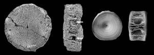
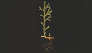
Other plants found in the Rhynie Chert have a range of different vascular systems. Asteroxylon, for example, already has xylem and phloem. © The Trustees of the Natural History Museum, London

A research group at The University of New Mexico has identified how an unusual prehistoric plant may provide new ways to interpret Earth’s ancient climate conditions.

Led by UNM Earth and Planetary Sciences Professor Zachary Sharp, the team published its findings in the Proceedings of the National Academy of Sciences (PNAS). The study, titled “Extreme triple oxygen isotope fractionation in Equisetum,” examines horsetails, which are hollow-stemmed plants that have existed on the planet for more than 400 million years. The researchers discovered that as water moves through these plants, it experiences such intense natural filtration that its oxygen isotope signatures become similar to those seen in meteorites or other extraterrestrial materials.

“It’s a meter-high cylinder with a million holes in it, equally spaced. It’s an engineering marvel,” Sharp said. “You couldn’t create anything like this in a laboratory.”

Unusual Isotope Behavior Reveals a New Climate Tool

The team’s results help clarify long-standing puzzles involving oxygen isotope measurements in desert plants and introduce a valuable method for reconstructing climate in dry regions.

Oxygen isotopes function as tracers, allowing scientists to learn about water sources, plant transpiration, and atmospheric moisture. Heavier isotopes are rare, which makes it challenging to predict how their ratios shift under real environmental conditions.

To investigate this process, Sharp’s group collected smooth horsetails (Equisetum laevigatum) along the Rio Grande in New Mexico. They tracked how oxygen isotope values changed from the lower sections of the plants to the upper portions. The highest samples produced extreme readings that previously appeared to fall outside any known Earth-based range.

Meteorite-Like Signatures Draw Global Attention

Sharp presented the work at the Goldschmidt Geochemistry Conference in Prague this past July.

“If I found this sample, I would say this is from a meteorite,” Sharp said during the conference. “But in fact, these values do go down to these crazy low levels.”

The newly collected data allowed the researchers to update their models, helping explain unusual isotope results found in other desert species. Sharp believes these refined models could also help scientists better understand ancient climate behavior.

Fossil Records Preserve Humidity From the Age of Dinosaurs

Fossil horsetails, which once grew up to 30 meters tall, contain tiny silica particles called phytoliths. These structures may retain isotope signatures for millions of years. According to Sharp, the phytoliths work as a “paleo-hygrometer,” or a way to measure ancient humidity.

“We can now begin to reconstruct the humidity and climate conditions of environments going back to when dinosaurs roamed the Earth,” he said.

This research expands UNM’s contributions to the geosciences and highlights horsetails, some of the planet’s oldest surviving plants, as unexpected yet powerful record keepers of Earth’s climate history.

Reference:

Zachary Sharp, Jordan Wostbrock, Anthony Gargano, Vincent Hare, Jessica Johnson, Thure Cerling, Payal Banerjee, Catherine Peshek, Cloe Knutson, Lauren Hartzell, Erick Cano, Elena Stiles, Kelley R. Bassett, Kira Holland, Michael H. Dowd, Jarunetr (Nadia) Sae-Lim, Teresa Dominguez, Dalton Bryant, Eduardo Di Marcantonio, Jensen Wainwright, Maxwell Horsford, Paul Botté, Catherine Gagnon, Paula J. Rudall, James Ehleringer. Extreme triple oxygen isotope fractionation in Equisetum. Proceedings of the National Academy of Sciences, 2025; 122 (44) DOI: 10.1073/pnas.2507455122

Note: The above post is reprinted from materials provided by University of New Mexico.

What Is the Cause of an Earthquake?

Seismogram
Representative Image: Seismogram

What Is the Cause of an Earthquake? Understanding Earthquake Origins in Geology

The cause of an earthquake lies in the sudden release of stored elastic energy within the Earth’s crust or upper mantle. This energy is generated by tectonic forces that slowly deform rocks over time until they exceed their mechanical strength. When failure occurs, rocks rupture along faults, releasing energy in the form of seismic waves that propagate through the Earth—what we experience as an earthquake.

From a geological perspective, earthquakes are not random events. They are the direct result of plate tectonics, stress accumulation, rock mechanics, and fault behavior, operating over timescales ranging from seconds to millions of years.

The Fundamental Geological Cause of Earthquakes

At the most basic level, earthquakes are caused by brittle failure of rocks under stress.

Stress Accumulation in the Earth’s Crust

Stress builds up in rocks due to:

  • Plate motion
  • Gravitational loading
  • Thermal expansion
  • Isostatic adjustment

Three principal stresses act on rocks:

  • σ₁ – maximum principal stress
  • σ₂ – intermediate principal stress
  • σ₃ – minimum principal stress

As tectonic plates move, stress accumulates along zones of weakness—primarily faults.

Elastic Deformation and Rock Failure

Rocks behave elastically under low stress, meaning they deform but return to their original shape. When stress exceeds the rock’s elastic limit, brittle failure occurs, producing:

  • Fractures
  • Fault slip
  • Sudden energy release

This process is governed by the Mohr–Coulomb failure criterion, a fundamental principle in rock mechanics.

Faults as the Primary Source of Earthquakes

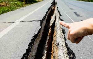
Most earthquakes occur along geological faults, which are fractures with measurable displacement.

Fault Locking and Stick–Slip Behavior

Faults are not continuously moving. Instead, they often remain locked due to friction. As tectonic motion continues, stress accumulates until:

  • Frictional resistance is overcome
  • Sudden slip occurs
  • Stored elastic strain is released

This behavior is known as the elastic rebound theory, first proposed by H. F. Reid after the 1906 San Francisco earthquake.

Types of Faults That Generate Earthquakes

Different fault types produce earthquakes under different stress regimes:

  • Normal faults → extensional stress
  • Reverse and thrust faults → compressional stress
  • Strike-slip faults → shear stress

The type of fault controls:

  • Earthquake depth
  • Rupture geometry
  • Surface deformation
  • Seismic hazard

Plate Tectonics and Earthquake Generation

Plate tectonics provides the global framework for understanding earthquake causes.

Convergent Plate Boundaries

At convergent boundaries, plates collide, producing:

  • Subduction-zone earthquakes
  • Deep-focus earthquakes (up to 700 km)
  • Some of the largest earthquakes on Earth

These earthquakes occur due to megathrust faulting, where one plate is forced beneath another.

Divergent Plate Boundaries

At divergent boundaries:

  • Plates move apart
  • Normal faulting dominates
  • Earthquakes are generally shallow and moderate in magnitude

These are common at mid-ocean ridges and continental rifts.

Transform Plate Boundaries

Transform boundaries accommodate horizontal motion:

  • Strike-slip faulting
  • Shallow but potentially destructive earthquakes

These boundaries produce frequent seismic activity due to high strain rates.

Earthquake Focus, Epicenter, and Seismic Energy Release

Focus (Hypocenter)

The focus is the point inside the Earth where rupture begins. It represents the true origin of the earthquake.

Epicenter

The epicenter is the point on Earth’s surface directly above the focus. Damage is often greatest near the epicenter, but this depends on depth and local geology.

Seismic Waves

Earthquake energy travels as:

  • P-waves (compressional)
  • S-waves (shear)
  • Surface waves (Love and Rayleigh)

Surface waves cause the most damage, as they have large amplitudes near the surface.

Secondary Geological Causes of Earthquakes

While tectonics dominate, other geological processes can also cause earthquakes.

Volcanic Earthquakes

Volcanic activity generates earthquakes due to:

  • Magma movement
  • Gas pressure changes
  • Rock fracturing

These earthquakes are typically shallow and localized.

Isostatic Adjustment Earthquakes

Post-glacial rebound causes earthquakes as the crust responds to unloading after ice-sheet melting. These are common in formerly glaciated regions.

Landslide-Induced Earthquakes

Large landslides or rock avalanches can generate seismic signals, although they are not tectonic in origin.

Human-Induced (Anthropogenic) Earthquakes

Some earthquakes are caused or triggered by human activities.

Reservoir-Induced Seismicity

Large dams alter stress and pore pressure in the crust, sometimes triggering earthquakes.

Fluid Injection and Extraction

Activities such as:

  • Wastewater injection
  • Hydraulic fracturing
  • Geothermal energy extraction

can increase pore pressure, reducing fault friction and triggering seismic events.

Mining-Induced Seismicity

Underground mining redistributes stress, sometimes causing rockbursts and seismic events.

Why Earthquakes Occur Suddenly

Strain Energy Storage

Tectonic motion is slow—typically millimeters per year—but strain accumulates over decades to centuries.

Sudden Stress Release

Once frictional resistance is exceeded, rupture occurs in seconds, releasing:

  • Seismic energy
  • Heat
  • Permanent displacement

This contrast between slow buildup and rapid release explains the sudden nature of earthquakes.

Earthquake Magnitude, Energy, and Rupture Area

The size of an earthquake depends on:

  • Fault area that ruptures
  • Amount of slip
  • Rock rigidity

Large earthquakes involve long fault segments and high slip values, while small earthquakes rupture limited areas.

Geological Conditions That Amplify Earthquake Effects

Earthquake damage is not controlled solely by magnitude.

Local Geology

Soft sediments amplify seismic waves, increasing damage.

Fault Proximity

Shallow earthquakes near populated areas are more destructive.

Basin Effects

Sedimentary basins can trap and amplify seismic waves.

Why Earthquakes Cannot Yet Be Predicted

Although the cause of earthquakes is well understood, exact prediction remains impossible because:

  • Stress is heterogeneous
  • Fault friction varies
  • Subsurface conditions are complex

Modern seismology focuses on probabilistic hazard assessment, not deterministic prediction.

References

  • Reid, H. F. (1910). The Mechanics of the Earthquake. Carnegie Institution of Washington.
  • Scholz, C. H. (2019). The Mechanics of Earthquakes and Faulting. Cambridge University Press.
  • Anderson, E. M. (1951). The Dynamics of Faulting and Dyke Formation. Oliver & Boyd.
  • Kanamori, H., & Brodsky, E. E. (2004). “The physics of earthquakes.” Reports on Progress in Physics, 67, 1429–1496.
  • Turcotte, D. L., & Schubert, G. (2014). Geodynamics. Cambridge University Press.
  • Shearer, P. M. (2009). Introduction to Seismology. Cambridge University Press.

What Are the Different Types of Faults in Geology?

Different Types of Faults

Types of Faults in Geology — How Earth’s Crust Breaks, Moves, and Evolves

In geology, faults are fractures or zones of fractures in the Earth’s crust along which measurable displacement has occurred. The study of faults is central to structural geology, tectonics, seismology, and engineering geology, because faults control mountain building, basin formation, earthquakes, and the mechanical behavior of the lithosphere.

Understanding the types of faults allows geologists to interpret:

  • Regional and global stress regimes
  • Plate tectonic environments
  • Earthquake mechanisms and hazards
  • Crustal deformation through geological time

Faults are classified primarily based on the direction of movement, orientation of the fault plane, and the stress field responsible for deformation.

Faults, Stress, and Rock Mechanics — The Physical Basis

Before classifying faults, it is essential to understand the three principal stresses acting on rocks:

  • σ₁ (maximum principal stress)
  • σ₂ (intermediate stress)
  • σ₃ (minimum principal stress)

Faulting occurs when applied stress exceeds the shear strength of rocks, as described by the Mohr–Coulomb failure criterion. The orientation of σ₁ and σ₃ determines how rocks break and slide, directly controlling the type of fault that forms.

Main Types of Faults in Geology

Geological faults are grouped into four fundamental categories, each linked to a specific tectonic stress regime.

1. Normal Faults

A normal fault forms when the crust is subjected to extensional stress, causing it to stretch and thin. In a normal fault, the hanging wall moves downward relative to the footwall.

Key Characteristics

  • Associated with tensional (extensional) stress
  • Hanging wall moves down
  • Fault plane typically dips 45–70°
  • Produces fault scarps and horst–graben systems

Geological Settings

  • Continental rift zones
  • Mid-ocean ridges
  • Back-arc basins

Geological Significance

Normal faults accommodate crustal extension and are fundamental to the formation of rift valleys and sedimentary basins.

Examples

  • East African Rift System
  • Basin and Range Province (USA)

Normal faulting dominates regions where σ₃ is vertical and σ₁ is horizontal.

2. Reverse Faults

A reverse fault develops under compressional stress, where the hanging wall moves upward relative to the footwall.

Key Characteristics

  • Compression shortens and thickens the crust
  • Hanging wall moves up
  • Fault plane dips steeply (>45°)
  • Commonly associated with folding

Geological Settings

  • Convergent plate boundaries
  • Continental collision zones
  • Active orogenic belts

Reverse faults are crucial indicators of crustal shortening and are often associated with large-scale mountain building.

3. Thrust Faults (Low-Angle Reverse Faults)

A thrust fault is a special type of reverse fault with a low dip angle, typically less than 30°. Thrust faults can transport rock masses tens to hundreds of kilometers.

Key Characteristics

  • Low-angle fault plane
  • Older rocks may overlie younger rocks
  • Formation of nappes and duplex structures

Geological Importance

Thrust faults are dominant in fold-and-thrust belts and represent some of the most dramatic crustal displacements on Earth.

Examples

  • Himalaya thrust systems
  • Alps and Zagros Mountains

Thrusting reflects a stress regime where σ₁ is horizontal and σ₃ is vertical.

4. Strike-Slip Faults

A strike-slip fault is characterized by horizontal movement parallel to the fault’s strike, driven by shear stress.

Subtypes of Strike-Slip Faults

Right-Lateral (Dextral) Faults
The opposite block moves to the right.

Left-Lateral (Sinistral) Faults
The opposite block moves to the left.

Key Characteristics

  • Vertical or near-vertical fault plane
  • Horizontal displacement dominates
  • Linear valleys, offset streams, sag ponds

Tectonic Settings

  • Transform plate boundaries
  • Continental shear zones

Examples

  • San Andreas Fault (USA)
  • Alpine Fault (New Zealand)

Strike-slip faulting reflects a stress regime where σ₁ and σ₃ are horizontal.

Oblique-Slip Faults

An oblique-slip fault combines vertical and horizontal movement, meaning both dip-slip and strike-slip components are present.

Why Oblique Faults Are Common
Natural stress fields are rarely perfectly aligned, so many faults record mixed displacement.

Geological Significance
Oblique-slip faults are common along:

  • Oblique plate boundaries
  • Continental margins
  • Reactivated ancient faults

Fault Zones vs Single Fault Planes

In reality, most faults are not single surfaces but fault zones, consisting of:

  • Multiple fault strands
  • Fracture networks
  • Fault breccia
  • Fault gouge

These zones may be meters to kilometers wide and strongly influence fluid flow, mineralization, and seismic behavior.

Special Fault Types in Structural Geology

Listric Faults
Curved normal faults that flatten with depth, common in sedimentary basins.

Growth Faults
Active during sediment deposition, producing thickened strata on the downthrown side.

Detachment Faults
Large, low-angle normal faults associated with crustal extension.

Blind Faults
Do not reach the surface but can still generate large earthquakes.

Faults and Earthquakes

Earthquakes occur when accumulated elastic strain is suddenly released along faults.

  • Normal faults → shallow extensional earthquakes
  • Reverse/thrust faults → large, destructive earthquakes
  • Strike-slip faults → lateral rupture and surface offsets

Fault geometry and slip rate control earthquake magnitude and frequency.

How Geologists Identify and Study Faults

Faults are analyzed using multiple complementary approaches:

  • Field mapping (slickensides, offsets, breccias)
  • Seismic reflection and refraction
  • Remote sensing and LiDAR
  • Paleoseismology
  • Microstructural analysis

Each method helps constrain fault kinematics and evolution.

Engineering and Environmental Importance of Fault Types

Fault classification directly affects:

  • Tunnel alignment and support design
  • Dam and foundation safety
  • Groundwater flow and contamination pathways
  • Landslide susceptibility
  • Seismic hazard assessment

Faults often act as barriers or conduits for fluids, depending on their internal structure.

References

  1. Anderson, E. M. (1951). The Dynamics of Faulting and Dyke Formation. Oliver & Boyd.
  2. Twiss, R. J., & Moores, E. M. (2007). Structural Geology. W.H. Freeman.
  3. Scholz, C. H. (2019). The Mechanics of Earthquakes and Faulting. Cambridge University Press.
  4. Fossen, H. (2016). Structural Geology. Cambridge University Press.
  5. Sibson, R. H. (1977). “Fault rocks and fault mechanisms.” Journal of the Geological Society, 133, 191–213.
  6. Davis, G. H., Reynolds, S. J., & Kluth, C. F. (2012). Structural Geology of Rocks and Regions. Wiley.

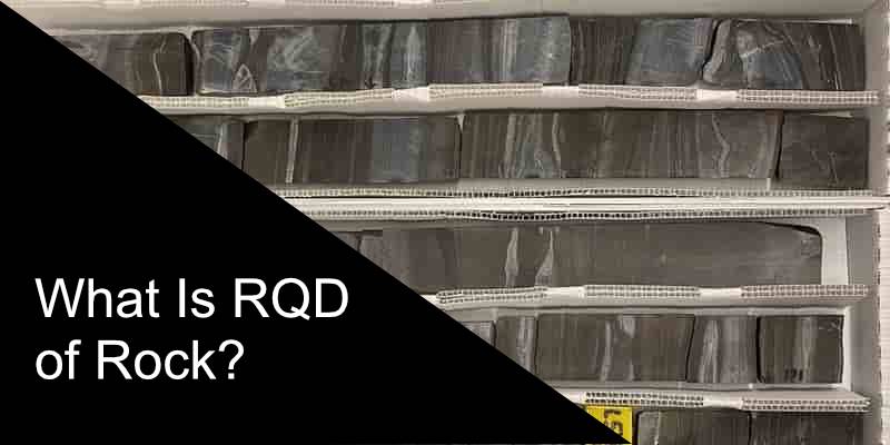
What Is RQD of Rock?

What Is RQD of Rock?

What Is RQD of Rock? Understanding Rock Quality Designation in Engineering Geology

RQD of rock, short for Rock Quality Designation, is a quantitative index used in engineering geology and rock mechanics to assess the degree of jointing and fracturing in a rock mass based on drill core recovery. Introduced by D. U. Deere (1963), RQD rapidly became a standard descriptor for evaluating rock mass quality in tunnels, foundations, slopes, dams, and underground excavations.

At its core, RQD answers a simple, practical question: How intact is the rock mass at the scale relevant to engineering works? By converting observations from drill cores into a percentage, RQD provides a repeatable, field-based metric that links geology to design decisions.

Definition of RQD (Rock Quality Designation)

Rock Quality Designation (RQD) is defined as the percentage of intact drill core pieces longer than 100 mm (10 cm) recovered from a core run, relative to the total length of that run.

RQD (%)= (∑length of core pieces ≥100 mm​/total core run length)×100

This definition deliberately filters out short, broken fragments, which are interpreted as evidence of fractures, joints, shears, or weathering within the rock mass.

Why RQD Matters in Engineering and Geology

RQD is not merely a descriptive number. It has direct engineering consequences because rock mass behavior—strength, deformability, permeability, and stability—is controlled far more by discontinuities than by intact rock strength alone.

RQD is widely used to:

  • Estimate rock mass quality at depth
  • Support tunnel and cavern design
  • Evaluate foundation conditions for dams and buildings
  • Assess slope stability and excavation safety
  • Feed into rock mass classification systems (RMR, Q-system)

In practice, RQD often represents the first quantitative bridge between geological logging and engineering design.

Historical Development of the RQD Concept

The RQD concept was proposed by Don U. Deere during the development of rock mechanics for large civil projects in the mid-20th century. Prior to RQD, core recovery alone was used, but recovery could be misleading—high recovery might still represent heavily fractured rock.

Deere recognized that fragment length distribution is a better proxy for rock mass integrity than total recovery. His 1963 work formalized RQD as a simple, field-applicable index that could be standardized across projects.

How RQD Is Measured — Step-by-Step Scientific Procedure

1. Core Drilling

RQD is measured using diamond drill cores, typically NX, HQ, or NQ sizes. Consistency in core diameter improves comparability.

2. Core Handling and Layout

Recovered core is carefully placed in core boxes in drilling order, preserving depth orientation.

3. Measuring Intact Core Pieces

Only core pieces ≥ 100 mm in length are counted. Measurements are made along the core axis, not end-to-end across fractures.

4. Calculating RQD

The summed length of qualifying pieces is divided by the core run length (often 1.0–3.0 m).

5. Reporting

RQD is reported as a percentage per run and sometimes averaged over intervals.

RQD Classification and Interpretation

RQD values are commonly interpreted using Deere’s original classification:

RQD (%) Rock Mass Quality
0–25 Very Poor
25–50 Poor
50–75 Fair
75–90 Good
90–100

Excellent

These categories are engineering descriptors, not absolute measures of strength. A rock mass with excellent RQD may still be weak if discontinuities are unfavorably oriented or infilled.

Geological Meaning of RQD Values

RQD is fundamentally a measure of fracture spacing and structural integrity:

  • High RQD (≥ 90%)
    Indicates widely spaced joints, massive or blocky rock, low deformation potential.
  • Moderate RQD (50–75%)
    Suggests moderately jointed rock with potential block instability.
  • Low RQD (< 50%)
    Reflects closely spaced fractures, shears, or weathered zones; typically problematic for excavation.

From a geological perspective, RQD indirectly reflects:

  • Tectonic history
  • Stress regimes
  • Degree of weathering
  • Lithological controls on fracture development

RQD vs Core Recovery — A Critical Distinction

A frequent misconception is equating core recovery with RQD.

  • Core Recovery measures how much core was recovered.
  • RQD measures how intact that recovered core is.

A core run may show 100% recovery but an RQD of 30%, indicating crushed or highly fractured rock. Conversely, moderate recovery with long intact pieces may yield high RQD.

This distinction is crucial in fault zones, shear zones, and weathered profiles.

RQD in Rock Mass Classification Systems

RQD is rarely used alone in modern engineering. Instead, it feeds into multi-parameter systems.

Rock Mass Rating (RMR)

In Bieniawski’s RMR system, RQD contributes up to 20 points, combined with:

  • UCS
  • Joint spacing
  • Joint condition
  • Groundwater
  • Orientation

Q-System (Barton et al.)

RQD appears directly in the numerator:

Q = RQD/Jn × Jr/Ja × Jw/SRF

Here, RQD represents the block size component of rock mass quality.

Engineering Applications of RQD

Tunnels and Underground Excavations

RQD guides:

  • Support type selection (rock bolts, shotcrete, lining)
  • Excavation method (TBM vs drill-and-blast)

Foundations

Low RQD zones may require:

  • Excavation replacement
  • Grouting
  • Design modification

Slopes and Open Excavations

RQD helps identify zones prone to:

  • Block failure
  • Toppling
  • Wedge instability

Limitations and Criticisms of RQD

Despite its usefulness, RQD has well-documented limitations:

  1. Orientation Bias
    RQD depends on drill direction relative to joint orientation. A borehole parallel to joints may overestimate quality.
  2. Ignores Joint Properties
    RQD does not account for:
    – Joint roughness
    – Aperture
    – Infilling
    – Persistence
  3. Insensitive to Lithology
    Strong and weak rocks may yield similar RQD values.
  4. Scale Dependency
    RQD reflects conditions at the borehole scale, not necessarily the excavation scale.

For these reasons, RQD should always be used in conjunction with detailed structural logging and geotechnical testing.

Advances Beyond Classical RQD

Modern practice supplements RQD with:

  • Fracture frequency (P10) from scanlines
  • Digital core scanning
  • Image-based discontinuity analysis
  • Rock mass block volume estimation

Nevertheless, RQD remains a globally accepted baseline index, especially in early-stage site investigations.

References

  1. Deere, D. U. (1963). Technical description of rock cores for engineering purposes. Rock Mechanics and Engineering Geology, 1, 16–22.
  2. Deere, D. U., & Deere, D. W. (1988). The Rock Quality Designation (RQD) Index in Practice. Rock Classification Systems for Engineering Purposes, ASTM STP 984.
  3. Bieniawski, Z. T. (1989). Engineering Rock Mass Classifications. Wiley.
  4. Barton, N., Lien, R., & Lunde, J. (1974). Engineering classification of rock masses for the design of tunnel support. Rock Mechanics, 6, 189–236.
  5. Palmström, A. (2005). Measurements of and correlations between block size and rock quality designation (RQD). Tunnelling and Underground Space Technology, 20, 362–377.
  6. Hoek, E., & Brown, E. T. (1997). Practical estimates of rock mass strength. International Journal of Rock Mechanics and Mining Sciences, 34(8), 1165–1186.

Intrusive Igneous Bodies: Types, Characteristics & Geological Processes

Types of Intrusive Igneous Bodies

Understanding Intrusive Igneous Bodies — How Magma Shapes the Earth’s Crust

Intrusive igneous bodies are masses of crystallized igneous rock that form when magma solidifies beneath Earth’s surface. These bodies, known collectively as plutonic bodies or plutons, cool slowly underground, resulting in coarse-grained, crystalline textures typical of rocks such as granite, diorite, gabbro, and tonalite. Because they form in the subsurface, intrusive bodies preserve critical records of magmatic processes, tectonic settings, crustal evolution, and thermal history (Best & Christiansen, 2001).

Intrusive igneous bodies vary enormously in size, geometry, depth of emplacement, and relationship with surrounding rock. Understanding their types is fundamental to:

  • Interpreting magmatic systems
  • Mapping tectonic environments
  • Reconstructing crustal evolution
  • Identifying mineral deposits
  • Understanding geothermal and volcanic systems

This article provides a comprehensive scientific overview of the main types of intrusive igneous bodies, integrating geological principles, petrology, structural geology, field relationships, and real scientific research.

What Defines an Intrusive Igneous Body?

An intrusive igneous body forms when magma intrudes into pre-existing rocks and cools in the crust, becoming plutonic rock. The key characteristics include:

  • Slow cooling, producing large, visible crystals
  • Cross-cutting or concordant relationships with host rock
  • Contact metamorphism aureoles caused by heat
  • Distinctive textures (phaneritic, porphyritic, pegmatitic)
  • Mappable geometry, allowing classification into types

The morphology of intrusive bodies depends on:

  • Magma viscosity
  • Tectonic stress regime
  • Depth of emplacement
  • Composition & temperature
  • Mechanical properties of the host rock

Major Types of Intrusive Igneous Bodies

Below is a systematic, scientifically grounded explanation of all major intrusive body types, integrating structural relationships and magmatic processes.

1. Batholiths — The Largest Intrusive Bodies

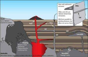
Batholiths are massive, composite intrusive complexes larger than 100 km², formed by the amalgamation of multiple plutons over millions of years.

Key Characteristics

  • Irregular shape
  • Composed mainly of granitic to dioritic rocks
  • Represent continental arc magmatism (subduction zones)
  • Display zonation: mafic at margins → felsic at center
  • Form deep in the crust (5–30 km depth)

Geological Significance

Batholiths reflect long-lived magmatic arcs associated with orogenies.

Examples

  • Sierra Nevada Batholith (USA)
  • Andean Coastal Batholith (Peru & Chile)

Research indicates batholiths form through successive pulses of magma rather than single emplacement events (Paterson et al., 1994).

2. Plutons — Discrete Intrusive Bodies

A pluton is any large, blob-like intrusive body that crystallizes underground. Plutons may be:

  • Granite plutons (felsic)
  • Gabbro plutons (mafic)
  • Diorite plutons (intermediate)

Most plutons are sub-batholithic, meaning they may later join others to form a batholith.

Field Indicators

  • Coarse-grained texture
  • Sharp or diffuse intrusive contacts
  • Contact metamorphic aureoles

3. Stocks — Smaller Plutons

A stock is a small pluton less than 100 km² in surface exposure. Stocks often represent the upper tips of larger batholiths.

They show similar textures and mineralogy to plutons but are more restricted spatially.

4. Dikes — Vertical or Steeply Inclined Intrusions

Dikes (or dykes) are discordant tabular intrusions cutting across pre-existing structures.

Key Features

  • Steep or vertical orientation
  • Fine to medium grain size (faster cooling)
  • Often form swarm systems (parallel or radiating groups)
  • Transport magma upward during volcanic activity

Dikes record extensional tectonics, such as:

  • Rift zones
  • Mid-ocean ridges
  • Large Igneous Provinces (LIPs)

Example

  • The Mackenzie Dyke Swarm (Canada) — the world’s largest dyke swarm.

5. Sills — Horizontal or Gently Inclined Intrusions

A sill is a tabular, concordant intrusive body that injects parallel to sedimentary bedding or metamorphic foliation.

Characteristics

  • Typically forms under low differential stress
  • May feature columnar jointing
  • Can cause significant contact metamorphism in overlying strata

Sills commonly occur in continental flood basalt provinces, such as:

  • Karoo Sill Complex (South Africa)
  • Palatine Sill (Scotland)

6. Laccoliths — Dome-Shaped Intrusions

A laccolith forms when magma injects between rock layers and pushes the overlying strata upward, forming a dome.

Features

  • Flat base, convex upper surface
  • Viscous, silica-rich magma (e.g., rhyolite)
  • Found in shallow crustal levels

This intrusion geometry requires higher magma pressure than sills.

Classic Example

  • Henry Mountains Laccoliths (USA) — studied by Grove Karl Gilbert (1877), foundational to intrusion mechanics.

7. Lopoliths — Saucer-Shaped Intrusions

Lopoliths are large, bowl-shaped intrusive bodies that depress underlying strata.

Characteristics

  • Concave-up geometry
  • Often associated with mafic magmatism
  • Form under extensional tectonics

Notable Example

  • Bushveld Complex (South Africa) — the world’s largest layered mafic intrusion.

8. Pipes and Diatremes — Volcanic Conduits

These cylindrical intrusions represent vertical channels through which magma ascends.

Types:

  • Volcanic pipes — ultramafic to kimberlite; may host diamonds
  • Diatremes — explosive breccia-filled conduits

Pipes provide direct windows into deep mantle-derived magmas.

9. Pegmatites — Extremely Coarse-Grained Intrusions

Pegmatites form from volatile-rich late-stage magmas, yielding giant crystals of:

  • Feldspar
  • Quartz
  • Micas
  • Rare earth minerals (Li, Ta, Nb)

Pegmatites are essential for critical mineral resources used in batteries and electronics.

10. Xenolith-Bearing Intrusions

Some intrusive bodies transport xenoliths, fragments of country rock or mantle material.

These xenoliths serve as samples of inaccessible crustal and mantle layers, aiding in geochemical modeling (Hawkesworth & Kemp, 2006).

How Intrusive Bodies Interact with Surrounding Rocks

When magma intrudes, it alters nearby rocks via contact metamorphism, producing:

  • Chilled margins (rapid cooling)
  • Metamorphic aureoles
  • Skarns (fluid–rock reactions)

The thermal gradient and time duration determine metamorphic grade.

Textural and Mineralogical Indicators of Intrusive Emplacement

Intrusive igneous bodies exhibit diagnostic textures, including:

Phaneritic Texture

Large, interlocking crystals formed during slow cooling.

Porphyritic Texture

Large phenocrysts set in a finer groundmass.

Graphic Texture

Intergrowth of quartz and feldspar in pegmatites.

Zoned Minerals

Reflect changing magmatic conditions during crystallization.

How Geologists Identify and Study Intrusive Igneous Bodies

Field Mapping

Noting cross-cutting relationships and intrusive contacts.

Petrography

Microscopic analysis of crystal textures and mineral assemblages.

Geochemical Signatures

Trace elements and isotopes reveal source magmas and crustal contamination.

Geochronology

Radiometric dating (U-Pb zircon) determines magma emplacement ages.

Geophysics

Gravity and magnetic surveys detect subsurface plutons and sills.

Frequently Asked Questions

What are intrusive igneous bodies?

They are rock masses formed when magma cools and solidifies beneath Earth’s surface.

What is the difference between a dike and a sill?

A dike is discordant and cuts across layers; a sill is concordant and forms parallel to them.

Which intrusive body is the largest?

Batholiths are the largest, exceeding 100 km² in surface exposure.

What is a laccolith vs. a lopolith?

A laccolith domes the overlying strata upward, while a lopolith depresses underlying strata downward.

How do intrusive bodies relate to tectonics?

They record magmatic processes linked to plate boundaries, rifts, and crustal thickening.

Key Takeaways

  1. Intrusive igneous bodies form when magma solidifies underground, producing coarse-grained rocks.
  2. Their morphology reflects pressure, viscosity, tectonic stress, and host-rock properties.
  3. Types include plutons, batholiths, stocks, dikes, sills, laccoliths, lopoliths, pipes, pegmatites, and more.
  4. These bodies reveal critical information about magmatism, crustal growth, mineralization, and tectonic evolution.
  5. Field observations, petrography, isotopes, and geophysics are essential tools for their study.

References

  1. Best, M. G., & Christiansen, E. H. (2001). Igneous Petrology. Blackwell Science.
  2. Paterson, S. R., et al. (1994). “Magmatic processes in batholith construction.” Journal of Structural Geology, 16(11), 1675–1693.
  3. Gilbert, G. K. (1877). Report on the Geology of the Henry Mountains. U.S. Geological Survey.
  4. Hawkesworth, C. J., & Kemp, A. I. S. (2006). “Evolution of the continental crust.” Nature, 443, 811–817.
  5. Winter, J. D. (2010). Principles of Igneous and Metamorphic Petrology. Pearson.
  6. Wilson, M. (1989). Igneous Petrogenesis. Springer.

Geological Formation: Definition, Origins, Processes, and Importance | Complete Geological Guide

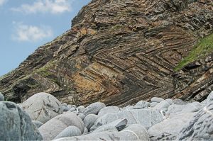
The ripplocation phenomenon can help explain the behavior of materials when they bend and break — everything from a nanoscale material to massive geological formations.

What Is a Geological Formation? A Scientific, Stratigraphic, and Geochemical Explanation

A geological formation is a fundamental unit of stratigraphy used to describe a body of rock with consistent lithological characteristics that distinguish it from adjacent rock layers. In essence, a geological formation is a mappable, identifiable package of rock that formed under specific geological conditions and environments (North American Commission on Stratigraphic Nomenclature, 2005).

Formations may consist of sedimentary, igneous, or metamorphic rocks, and they represent a natural chapter in Earth’s geological history — a period when certain environmental, tectonic, depositional, or magmatic conditions prevailed.

Formal Definition of a Geological Formation

In stratigraphy, a formation is defined as:

“A lithologically distinctive stratigraphic unit that is large enough to be mapped at the Earth’s surface or traced in the subsurface.”
(International Stratigraphic Guide, Salvador 1994)

Key Characteristics:

  • Distinct lithology (rock type, color, grain size, mineralogy)
  • Clear boundaries that can be mapped
  • Internal consistency within the rock body
  • Represents a specific geological environment or process

A formation is the basic building block of the geological column, and multiple formations may group together into members (smaller units) or groups (larger units).

Why Geological Formations Matter

Formations are essential because they allow geologists to:

1. Reconstruct Earth’s History

Formations preserve evidence of:

  • Ancient seas
  • Volcanic eruptions
  • Mountain-building events
  • Climate shifts
  • Biological evolution

2. Interpret Past Environments (Paleoenvironmental Reconstruction)

Sedimentary structures and fossils inside formations reveal:

  • River systems
  • Deserts
  • Glacial environments
  • Coral reefs
  • Deep-sea basins

3. Identify Natural Resources

Many resources occur within specific formations, including:

  • Groundwater aquifers (e.g., sandstone formations)
  • Petroleum reservoirs (carbonate & sandstone formations)
  • Ore deposits (volcanogenic or metamorphosed formations)

4. Support Engineering and Construction

Engineers use formations to evaluate:

  • Bedrock stability
  • Slope stability
  • Foundation design
  • Earthquake risk

How Geological Formations Develop — The Science Behind Their Origins

The development of geological formations depends on the type of rock involved. Below is a detailed breakdown from a geological processes perspective.

Sedimentary Formations

Sedimentary formations arise from the accumulation, compaction, and cementation of sediments over time. They cover about 75% of the Earth’s continents’ surface (Blatt, Middleton & Murray, 1980).

Controls on Sedimentary Formation Creation

1- Depositional Environment

  • Marine (continental shelf, deep sea)
  • Fluvial (river channels, floodplains)
  • Aeolian (dunes)
  • Lacustrine (lakes)

2- Sediment Supply & Transport

  • Weathering
  • Erosion
  • River transport
  • Oceanic currents

3- Sea-Level Changes
Transgression/regression cycles create distinct mappable formations.

4- Diagenesis
Cementation and chemical changes solidify the rock.

Example of a Sedimentary Formation:

The Navajo Sandstone (USA) — famous for its cross-bedded dunes and pale orange colors, representing an ancient Jurassic desert environment.

Igneous Formations

Igneous geological formations develop from magma crystallization (intrusive) or lava solidification (extrusive).

Key Igneous Processes Influencing Formations

  • Cooling rate influences crystal size
  • Magma composition (mafic, intermediate, felsic)
  • Tectonic setting (subduction zones, mid-ocean ridges, hotspots)

Examples:

  • Deccan Traps (India) — basaltic flood lavas
  • Skaergaard Intrusion (Greenland) — layered mafic intrusion crucial for igneous petrology research (Wager & Brown, 1968)

Metamorphic Formations

Metamorphic formations arise when existing rocks transform under:

  • Heat
  • Pressure
  • Chemically active fluids

These processes occur during:

  • Mountain-building (orogeny)
  • Subduction
  • Crustal thickening

Types of Metamorphism Shaping Formations

  • Regional metamorphism — large-scale, tectonic
  • Contact metamorphism — due to magma intrusions
  • Hydrothermal alteration — mineralization and ore formation

Example:

The Scottish Highlands Metamorphic Complex, shaped by the Caledonian Orogeny.

Stratigraphy and Naming of Geological Formations

To be officially recognized, a formation must be:

  • Described in a scientific publication
  • Mapped at a mappable scale (1:25,000 or 1:50,000)
  • Defined at a type locality (“type section”)

Naming conventions usually follow:

Geographic location + dominant lithology
Example: Burgess Shale Formation

Examples of Famous Geological Formations Worldwide

Sedimentary

  • Grand Canyon Formations (USA) — showcase 2 billion years of stratigraphy
  • White Cliffs of Dover (UK) — Upper Cretaceous chalk

Igneous

  • Giant’s Causeway (Northern Ireland) — columnar basalt
  • Siberian Traps (Russia) — massive volcanic province linked to mass extinction

Metamorphic

  • Himalayan Metamorphic Core — high-grade gneisses and migmatites

How Geologists Study Geological Formations

1. Field Mapping

Measuring layers, rock types, structures.

2. Petrographic Analysis

Microscopic examination of minerals.

3. Geochemical Techniques

Isotope analysis (Sr, Nd, Pb isotopes), elemental composition.

4. Geochronology

Radiometric dating (U-Pb, Ar-Ar) determines formation ages.

5. Remote Sensing & GIS

Mapping formations using satellite imagery.

Geological Formation vs. Other Stratigraphic Units

Unit Description Relative Scale
Group Several formations Larger
Formation Primary mappable unit Standard
Member Sub-unit within a formation Smaller
Bed Smallest unit (single layer) Very small


References

  1. Salvador, A. (1994). International Stratigraphic Guide. Geological Society of America.
  2. North American Commission on Stratigraphic Nomenclature (2005). North American Stratigraphic Code. AAPG Bulletin.
  3. Blatt, H., Middleton, G., & Murray, R. (1980). Origin of Sedimentary Rocks. Prentice Hall.
  4. Wager, L. R., & Brown, G. M. (1968). Layered Igneous Rocks. W.H. Freeman.
  5. Tucker, M. E. (2001). Sedimentary Petrology: An Introduction to the Origin of Sedimentary Rocks. Blackwell Science.
  6. Winter, J. D. (2010). Principles of Igneous and Metamorphic Petrology. Pearson.

Scientists uncover the secret triggers of ‘impossible’ earthquakes

Stick-slip events in the earth cause damage like this, but limited data from these relatively rare earthquakes makes them difficult to model with machine learning. Transfer learning may provide a path to understanding when such deep faults slip. Credit: Dreamstime

Earthquakes in places like Utah (USA), Soultz-sous-Forêts (France), and Groningen (the Netherlands) seem puzzling to scientists because, according to geological theory, they shouldn’t be possible. In these regions, the shallow layers of the Earth’s crust are thought to behave in a way that strengthens faults when they begin to move. Textbooks suggest that this strengthening effect should prevent earthquakes from happening at all. Yet, tremors still occur in these supposedly stable zones. Researchers from Utrecht University set out to understand why. Their findings, recently published in Nature Communications, reveal that faults which have remained inactive for millions of years can accumulate extra stress over time. Eventually, that built-up pressure may be released in a single event. This insight is crucial for identifying safer areas for technologies such as geothermal energy extraction and underground energy storage.

“Faults can be found almost everywhere. Faults in the shallow subsurface are usually stable, so we do not expect shock movements to occur along them,” explains Dr. Ylona van Dinther, who led the study. Yet, surprisingly, seismic activity does take place within the first few kilometers beneath the surface — precisely where the ground is considered most stable. These shallow earthquakes are often linked to human activities such as drilling, extraction, or fluid injection. The question, then, is why faults that normally grow stronger when they move can suddenly weaken and slip, releasing energy as an earthquake.

Inactive faults and slow healing

Many human-induced earthquakes occur along ancient, inactive faults that have not shifted for millions of years. Although these faults remain still, the surfaces where the rocks meet slowly “heal” over time, becoming stronger. This gradual strengthening creates additional resistance. When that resistance is finally overcome, it can cause an abrupt acceleration along the fault. That acceleration produces an earthquake, even in regions that geological models label as stable.

Because areas like these have no long-term record of seismic activity, local communities are often unprepared. Buildings and infrastructure are not designed to handle the shaking. “Furthermore, these earthquakes take place at a depth where human activities occur, in other words, no more than several kilometres deep. That is considerably less deep than the majority of natural earthquakes.” This shallowness means that such quakes can cause more noticeable and potentially damaging ground movement.

One-time events that stabilize over time

Interestingly, the Utrecht team found that these earthquakes are one-off events. Once the accumulated stress is released, the fault settles into a new, more stable state. “As a result, there is no more earthquake activity at that spot,” says Van Dinther. “This means that, although the subsurface in such areas will not settle immediately after human operations stop, the strength of the earthquakes — including the maximum expected magnitude — will gradually decrease.” When a fault strengthens as it moves, its broken sections can slide more easily past one another afterward, acting as natural barriers that prevent larger earthquakes from forming. This means the overall risk can be revised downward, since the potential for stronger quakes diminishes once the fault has slipped.

Implications for sustainable subsurface use

The research has significant consequences for how we use and manage the Earth’s subsurface. It shows that even in regions considered geologically stable, earthquakes can occur under certain conditions — but only once per fault. After the initial event, the area tends to become more secure. Understanding how faults behave, how they “heal,” and what causes them to accelerate or slow down is essential for minimizing seismic risks associated with geothermal energy, carbon storage, and similar technologies. With new computational models, Utrecht University researchers are already working to refine these predictions and improve how one-time earthquake risks are communicated.

Reference:
Meng Li, Andre R. Niemeijer, Ylona van Dinther. Frictional healing and induced earthquakes on conventionally stable faults. Nature Communications, 2025; 16 (1) DOI: 10.1038/s41467-025-63482-3

Note: The above post is reprinted from materials provided by Utrecht University.

Earth is slowly peeling its continents from below, fueling ocean volcanoes

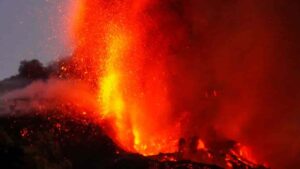
After five decades of dormancy, the Cumbre Vieja volcano on La Palma in the Canary Islands began erupting on Sept. 19, 2021. This image is from October 2021. Credit: Credit: Esteban Gazel/Provided

Earth scientists have uncovered a slow and surprising process beneath our planet’s surface that helps fuel volcanic activity in the oceans.

Researchers from the University of Southampton found that fragments of continents are gradually stripped away from below and drawn into the oceanic mantle — the hot, mostly solid layer beneath the sea floor that slowly circulates. Once there, this continental material can power volcanic eruptions for tens of millions of years.

This discovery resolves a long-standing geological puzzle: why certain ocean islands located far from tectonic plate boundaries contain chemical signatures that look distinctly continental, even though they lie in the middle of vast oceans.

The study, published in Nature Geoscience, was conducted by an international team from the University of Southampton, GFZ Helmholtz Centre for Geosciences in Potsdam, the University of Potsdam, Queen’s University (Canada), and Swansea University.

Ancient chemical clues deep within the mantle

Ocean islands such as Christmas Island in the northeast Indian Ocean often contain unusually high concentrations of certain “enriched” elements that typically come from continents. Scientists have compared this mixing process to the motion of a cake mixer folding in older, recycled ingredients from deep within the Earth.

For years, geologists assumed these enriched elements came from ocean sediments pulled into the mantle when tectonic plates sink, or from columns of rising hot rock known as mantle plumes.

However, those explanations have limits. Some volcanic regions lack evidence of recycled crust, while others seem too shallow and cool to be driven by deep mantle plumes.

“We’ve known for decades that parts of the mantle beneath the oceans look strangely contaminated, as if pieces of ancient continents somehow ended up in there,” said Thomas Gernon, Professor of Earth Science at the University of Southampton and the study’s lead author. “But we haven’t been able to adequately explain how all that continental material got there.”

Continents are peeling from below

The researchers propose a new mechanism: continents not only split apart at the surface but also peel away from below, and across far greater distances than scientists once believed possible.

To test this, the team built computer simulations that recreated how the mantle and continental crust behave when stretched by tectonic forces.

Their results show that when continents begin to break apart, powerful stresses deep within the Earth trigger a slow-moving “mantle wave.” This rolling motion travels along the base of the continents at depths of 150 to 200 kilometers, disturbing and gradually stripping material from their deep roots.

The process happens at an incredibly slow rate — roughly a millionth the speed of a snail. Over time, these detached fragments are carried sideways for more than 1,000 kilometers into the oceanic mantle, where they feed volcanic activity for tens of millions of years.

Study co-author Professor Sascha Brune of GFZ in Potsdam explained, “We found that the mantle is still feeling the effects of continental breakup long after the continents themselves have separated. The system doesn’t switch off when a new ocean basin forms — the mantle keeps moving, reorganizing, and transporting enriched material far from where it originated.”

Clues from the Indian Ocean

To support their model, the team analyzed chemical and geological data from regions such as the Indian Ocean Seamount Province — a chain of volcanic formations that appeared after the breakup of the supercontinent Gondwana over 100 million years ago.

Their findings show that soon after Gondwana split apart, a pulse of magma unusually rich in continental material erupted to the surface. Over time, this chemical signature gradually faded as the flow of material from beneath the continents diminished. Notably, this happened without the presence of a deep mantle plume, challenging long-held assumptions about the source of such volcanism.

Professor Gernon added: “We’re not ruling out mantle plumes, but this discovery points to a completely new mechanism that also shapes the composition of the Earth’s mantle. Mantle waves can carry blobs of continental material far into the oceanic mantle, leaving behind a chemical signature that endures long after the continents have broken apart.”

The research also builds on the team’s earlier work showing that these slow, rolling mantle waves can have dramatic effects deep inside continents. Their previous studies suggest that such waves may help trigger diamond eruptions and even reshape landscapes thousands of kilometers away from tectonic boundaries.

Reference:
T. M. Gernon, S. Brune, T. K. Hincks, M. R. Palmer, C. J. Spencer, E. J. Watts, A. Glerum. Enriched mantle generated through persistent convective erosion of continental roots. Nature Geoscience, 2025; DOI: 10.1038/s41561-025-01843-9

Note: The above post is reprinted from materials provided by University of Southampton.

World’s oldest RNA extracted from woolly mammoth

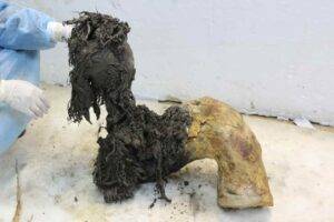
One of Yuka's legs, illustrating the exceptional preservation of the lower part of the leg after the skin had been removed, which enabled recovery of ancient RNA molecules. Photo credit: Valeri Plotnikov. Credit: Valeri Plotnikov
One of Yuka’s legs, illustrating the exceptional preservation of the lower part of the leg after the skin had been removed, which enabled recovery of ancient RNA molecules. Photo credit: Valeri Plotnikov. Credit: Valeri Plotnikov

Researchers from Stockholm University have—for the first time ever—managed to successfully isolate and sequence RNA molecules from Ice Age woolly mammoths. These RNA sequences are the oldest ever recovered and come from mammoth tissue preserved in the Siberian permafrost for nearly 40,000 years.

The study, published in the journal Cell, shows that not only DNA and proteins, but also RNA, can be preserved for very long periods of time, and provide new insights into the biology of species that have long since become extinct.

“With RNA, we can obtain direct evidence of which genes are ‘turned on,” offering a glimpse into the final moments of life of a mammoth that walked the Earth during the last Ice Age. This is information that cannot be obtained from DNA alone,” says Emilio Mármol, lead author of the study and formerly a postdoctoral researcher at Stockholm University.

He is now based at the Globe Institute in Copenhagen. During his time at Stockholm University, he teamed up with researchers at SciLifeLab and the Center for Palaeogenetics, a joint initiative between Stockholm University and the Swedish Museum of Natural History.

Sequencing prehistoric genes and studying how they are activated is important to understand the biology and evolution of extinct species. For years, scientists have been decoding mammoth DNA to piece together their genomes and evolutionary history.

Yet RNA, the molecule that shows which genes are active, has so far remained out of reach. The long-held belief that RNA is too fragile to even survive a few hours after death has likely discouraged researchers from exploring these information-rich molecules in mammoths and other long-extinct species.

“We gained access to exceptionally well-preserved mammoth tissues unearthed from the Siberian permafrost, which we hoped would still contain RNA molecules frozen in time,” adds Mármol.

“We have previously pushed the limits of DNA recovery past a million years. Now, we wanted to explore whether we could expand RNA sequencing further back in time than done in previous studies,” says Love Dalén, professor of Evolutionary Genomics at Stockholm University and the Center for Palaeogenetics.

The oldest RNA ever sequenced

The researchers were able to identify tissue-specific patterns of gene expression in frozen muscle remains from Yuka, a juvenile mammoth that died almost 40,000 years ago. Among the more than 20,000 protein-coding genes in the mammoth’s genome, far from all of them were active. The detected RNA molecules code for proteins with key functions in muscle contraction and metabolic regulation under stress.

“We found signs of cell stress, which is perhaps not surprising since previous research suggested that Yuka was attacked by cave lions shortly before his death,” says Mármol.

The researchers also found a myriad of RNA molecules that regulate the activity of genes in the mammoth muscle samples.

“RNAs that do not encode for proteins, such as microRNAs, were among the most exciting findings we got,” says Marc Friedländer, associate professor at the Department of Molecular Biosciences, The Wenner-Gren Institute at Stockholm University and SciLifeLab.

“The muscle-specific microRNAs we found in mammoth tissues are direct evidence of gene regulation happening in real time in ancient times. It is the first time something like this has been achieved,” he says.

The microRNAs that were identified also helped the researchers confirm that the findings really came from mammoths.

“We found rare mutations in certain microRNAs that provided a smoking-gun demonstration of their mammoth origin. We even detected novel genes solely based on RNA evidence, something never before attempted in such ancient remains,” notes Bastian Fromm, associate professor at the Arctic University Museum of Norway (UiT).

‘RNA molecules can survive much longer than previously thought’

“Our results demonstrate that RNA molecules can survive much longer than previously thought. This means that we will not only be able to study which genes are ‘turned on’ in different extinct animals, but it will also be possible to sequence RNA viruses, such as influenza and coronaviruses, preserved in Ice Age remains,” says Dalén.

In the future, the researchers hope to conduct studies that combine prehistoric RNA with DNA, proteins, and other preserved biomolecules.

“Such studies could fundamentally reshape our understanding of extinct megafauna as well as other species, revealing the many hidden layers of biology that have remained frozen in time until now,” concludes Mármol.

Reference:
Ancient RNA expression profiles from the extinct woolly mammoth, Cell (2025). DOI: 10.1016/j.cell.2025.10.025.

Note: The above post is reprinted from materials provided by Stockholm University

Oldest oceanic reptile ecosystem from the Age of Dinosaurs found on Arctic island

Earliest oceanic tetrapod ecosystem from 249 million years ago. A pod of the small-bodied ichthyopterygian ('fish-lizard') Grippia longirostris hunting squid-like ammonoids (top left). The marine amphibian Aphaneramma captures the bony fish Bobastrania (foreground). The gigantic ichthyosaur Cymbospondylus lurks in the depths (bottom right). Fossil of these ancient marine reptiles and amphibians are today preserved on the Arctic island of Spitsbergen in the Svalbard archipelago. Credit: Robert Back
Earliest oceanic tetrapod ecosystem from 249 million years ago. A pod of the small-bodied ichthyopterygian (‘fish-lizard’) Grippia longirostris hunting squid-like ammonoids (top left). The marine amphibian Aphaneramma captures the bony fish Bobastrania (foreground). The gigantic ichthyosaur Cymbospondylus lurks in the depths (bottom right). Fossil of these ancient marine reptiles and amphibians are today preserved on the Arctic island of Spitsbergen in the Svalbard archipelago. Credit: Robert Back

More than 30,000 teeth, bones and other fossils from a 249 million-year-old community of extinct marine reptiles, amphibians, bony fish and sharks have been discovered on the remote Arctic island of Spitsbergen. These record the earliest radiation of land-living animals into oceanic ecosystems following cataclysmic extinction and extreme global warming at the dawn of the Age of Dinosaurs.

The fossils were found in 2015, but took nearly a decade of painstaking work to excavate, prepare, sort, identify, and analyze. The long-awaited research findings have now been published by a team of Scandinavian paleontologists from the Natural History Museum at the University of Oslo, and the Swedish Museum of Natural History in Stockholm.

The paper is published in the journal Science.

Spitsbergen in the Svalbard archipelago is world famous for producing marine fossils from the beginning of the Age of Dinosaurs. These are preserved in rock layers that were once mud at the bottom of a sea stretching from mid-to-high paleolatitudes and bordering the immense Panthalassa super-ocean. Most spectacular are the remains of bizarre marine reptiles and amphibians that represent the earliest adaptive specialization of land-living animals for life in offshore habitats.

The aftermath of Earth’s greatest extinction

Textbooks suggest that this landmark evolutionary event took place after the most catastrophic mass extinction in Earth history, some 252 million years ago. Termed the end-Permian mass extinction, this “great dying” wiped out over 90% of all marine species, and was driven by hyper-greenhouse conditions, oceanic deoxygenation, and acidification linked to massive volcanic eruptions initiating the breakup of the ancient Pangaean supercontinent.

Timing the recovery of marine ecosystems after the end-Permian mass extinction is one of the most debated topics in paleontology today. The long-standing hypothesis is that this process was gradual, spanning some eight million years, and involved a stepwise evolutionary progression of amphibians and reptiles successively invading open marine environments. However, the discovery of the new and exceptionally rich fossil deposit on Spitsbergen has now upended this traditional view.

The Spitsbergen fossil deposit is so dense that it actually forms a conspicuous bonebed weathering out along the mountainside. This accumulated over a very short geological timeframe, and therefore provides unprecedented insights into the structure of marine communities from only a few million years after the end-Permian mass extinction. Stratigraphic dating has pinpointed the age of the Spitsbergen fossil bonebed to around 249 million years ago.

Revealing a rapid recovery and rich diversity

Careful collection of the remains from 1 m2 grids covering 36 m2 has also ensured that over 800 kg of fossils, including everything from tiny fish scales and shark teeth to giant marine reptile bones and even coprolites (fossilized feces) were recovered.

The Spitsbergen fossil bonebed reveals that marine ecosystems bounced back extremely rapidly, and had established complex food chains with numerous predatory marine reptiles and amphibians by as little as three million years after the end-Permian mass extinction. Most surprising is the sheer diversity of fully aquatic reptiles, which included archosauromorphs (distant relatives of modern crocodiles) and an array of ichthyosaurs (“fish-lizards”) ranging in size from small squid-hunters less than one meter long to gigantic apex-predators exceeding five meters in length.

A computer-based global comparative analysis of the various animal groups further highlights the Spitsbergen fossil bonebed as one of the most species-rich marine vertebrate (backboned animal) assemblages ever discovered from the dawn of the Age of Dinosaurs. It also suggests that the origins of sea-going reptiles and amphibians are much older than previously suspected, and likely even preceded the end-Permian mass extinction.

This ecosystem reset would have opened new feeding niches, and ultimately, laid the foundations for modern marine communities as we know them today.

Reference:
Aubrey J. Roberts, Earliest oceanic tetrapod ecosystem reveals rapid complexification of Triassic marine communities, Science (2025). DOI: 10.1126/science.adx7390.

Note: The above post is reprinted from materials provided by Swedish Museum of Natural History.

How algae helped some life outlast extinction

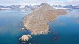
New research suggests that higher-latitude marine environments, such as those around the Selmaneset section in western Svalbard, seen here, may have provided a refuge for sea life during the Great Dying. Credit: Tereza Mosociova

Earth’s largest mass extinction occurred about 252 million years ago, wiping out the majority of marine and terrestrial life, disrupting the global carbon cycle for several hundred thousand years, and earning the title “the Great Dying.” Global warming, changing temperature gradients, shifts in nutrient cycling, and oxygen depletion wiped out 81% of all marine life at the time.

But cooler, relatively high latitude marine environments may have been refuges for species escaping volatile climate conditions elsewhere. S. Z. Buchwald and colleagues examined rock samples from the Arctic archipelago of Svalbard, Norway, and identified high levels of lipid biomarkers in rocks dated soon after the Permian-Triassic extinction.

Though the exact organism producing these molecules is unknown, it is likely a group of phytoplankton. This finding, published in AGU Advances, suggests that the cooler waters of the paleo-ocean allowed this primary producer to bloom and sustain remaining sea life.

The researchers collected 32 rock samples from Svalbard taken from layers formed pre- and postextinction and compared them with samples taken from other locations, such as northern Italy, southern China, and Türkiye. All represent warmer regions surrounding the prehistoric Tethys Ocean, a precursor to the modern Indian Ocean and Mediterranean Sea. The team examined the samples for C33–n-alkylcyclohexane (C33–n-ACH) and phytanyl toluene, molecular fossils that act like fingerprints of ancient marine life.

In the Svalbard samples dated after the Permian-Triassic extinction event, C33–n-ACH levels were 10 times higher than in samples from before the event. The researchers note that the preextinction samples likely experienced more degradation, but that alkylcyclohexane biomarkers are relatively resistant to such degradation, meaning the higher amounts detected after the extinction point to a true increase in the biomarker. In the samples taken from warmer regions, far less C33–n-ACH overall was detected, but a similar increase in abundance after the extinction event occurred.

Phytanyl toluene was largely absent from the Svalbard samples before the extinction and showed a similarly dramatic increase in the extinction’s aftermath. It was not present in the tropical samples, suggesting that it was produced by a different phytoplankton than the species that produced the C33–n-ACH.

Overall, these findings suggest that the phytoplankton producers of these biomarkers remained stable and thrived in cooler waters during a time when warmer waters were unable to support significant marine life, the researchers say.

Reference:
S. Z. Buchwald et al, Phytoplankton Blooms on the Barents Shelf, Svalbard, Associated With the Permian–Triassic Mass Extinction, AGU Advances (2025). DOI: 10.1029/2025av001785

Note: The above post is reprinted from materials provided by American Geophysical Union.

‘Weird’ new species of ancient fossil snake discovered in southern England

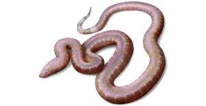
The new fossil snake species, Paradoxophidion richardoweni, lived in a much warmer England more than 37 million years ago. Credit: Jaime Chirinos

An extinct snake has slithered its way out of obscurity over four decades after its discovery. The newly described species of reptile, Paradoxophidion richardoweni, is offering new clues in the search for the origin of “advanced” snakes.

In 1981, the backbones of an ancient snake were uncovered at Hordle Cliff on England’s south coast. They’ve now been revealed as the remnants of a previously unknown species.

Research published in the journal Comptes Rendus Palevol has identified that the vertebrae belong to a new species named Paradoxophidion richardoweni. This animal would have lived around 37 million years ago, when England was home to a much wider range of snakes than it is now.

While little is known about this animal’s life, it could shed light on the early evolution of the biggest group of modern snakes. This is because Paradoxophidion represents an early-branching member of the caenophidians, the group containing the vast majority of living snakes.

The new species is so early in the evolution of the caenophidians that it has a peculiar mix of characteristics now found in different snakes throughout this group. This mosaic of features is summed up in its genus name, with Paradoxophidion meaning “paradox snake” in Greek.

Its species name, meanwhile, honors Richard Owen. Not only did he name the first fossil snakes found at Hordle Cliff, but this scientist was also instrumental in establishing what’s now the Natural History Museum where the fossils are cared for, giving the name multiple layers of meaning.

Lead author Dr. Georgios Georgalis, from the Institute of Systematics and Evolution of Animals of the Polish Academy of Sciences in Krakow, says that being able to describe a new species from our collections was “a dream come true.”

“It was my childhood dream to be able to visit the Natural History Museum, let alone do research there,” reveals Georgalis. “So, when I saw these very weird vertebrae in the collection and knew that they were something new, it was a fantastic feeling.”

“It’s especially exciting to have described an early diverging caenophidian snake, as there’s not that much evidence about how they emerged. Paradoxophidion brings us closer to understanding how this happened.”

What’s been discovered at Hordle Cliff?

Hordle Cliff, near Christchurch on England’s south coast, provides a window into a period of Earth’s history known as the Eocene that lasted from around 56 to 34 million years ago.

Dr. Marc Jones, our curator of fossil reptiles and amphibians who co-authored the research, says that this epoch saw dramatic climatic changes around the world.

“Around 37 million years ago, England was much warmer than it is now,” Jones explains. “Though the sun was very slightly dimmer, levels of atmospheric carbon dioxide were much higher.”

“England was also slightly closer to the equator, meaning that it received more heat from the sun year round.”

Fossils were first uncovered at Hordle Cliff around 200 years ago. In the early 1800s Barbara Rawdon-Hastings, the fossil-hunting Marchioness of Hastings, collected the skulls of crocodile relatives from the site, one of which Richard Owen would later name after her.

Since then, a variety of fossil turtles, lizards and mammals have also been uncovered at Hordle Cliff. There are also abundant snake fossils, including some particularly important species.

“The fossil snakes found at Hordle Cliff were some of the first to be recognized when Richard Owen studied them in the mid-nineteenth century,” says Georgalis. “They include Paleryx, the first named constrictor snake in the fossil record.”

“Smaller snakes from this site, however, haven’t been as well investigated. Paradoxophidion’s vertebrae are just a few millimeters long, so historically they’ve not had a lot of attention.”

To get a better look at these fossils, Jones and Georgalis took CT scans of the bones. In total, they identified 31 vertebrae from different parts of the spine of Paradoxophidion.

“We used these CT scans to make three-dimensional models of the fossils,” Jones adds. “These provide a digital record of the specimen, which we’ve shared online so that they can be studied by anyone, not just people who can come to the museum and use our microscopes.”

The scans show that the fossils are all slightly different shapes and sizes, as the snake’s spine bones gradually taper from head to tail. However, they share some features that show they all belong to one species.

Georgalis estimates that Paradoxophidion would have been less than a meter long, but other details about this animal’s life are hard to say. The lack of a skull makes it difficult to know what it ate, while the vertebrae don’t have any sign of being adapted for a specialized lifestyle, such as burrowing.

A living link to the past?

Though the vertebrae don’t give much away about Paradoxophidion’s lifestyle, they are strikingly similar to a group of snakes known as the Acrochordids. These reptiles are known as elephant trunk snakes due to their unusually baggy skin.

Today, only a few species of these snakes can be found living in southeast Asia and northern Australia. But they’re among the earliest branches of the caenophidian family tree, with a fossil record extending back over 20 million years.

“As Paradoxophidion is really similar to the acrochordids, it’s possible that this snake could be the oldest known member of this family,” muses Georgalis. “If it was, then it could mean that it was an aquatic species, as all Acrochordids are aquatic.”

“On the other hand, it might belong to a completely different group of caenophidians. There’s just not enough evidence at the moment to prove how this snake might have lived, or which family it belongs to.”

Finding out more about Paradoxophidion and the early evolution of the caenophidians means that more fossils will need to be studied. Georgalis hopes to continue his work in our fossil reptile collections in the near future, where he believes more new species might be waiting.

“I’m planning to study a variety of snake fossils in the collection, including those originally studied by Richard Owen” Georgalis adds. “These include the remains of the giant aquatic snake Palaeophis, which were first found in England in the nineteenth century.”

“There are also several bones with differing morphology that haven’t been investigated before that I’m interested in looking at. These might represent new taxa and offer additional clues about snake evolution.”

Reference:
Georgios L. Georgalis et al, A new peculiar early diverging caenophidian snake (Serpentes) from the late Eocene of Hordle Cliff, England, Comptes Rendus Palevol (2025). DOI: 10.5852/cr-palevol2025v24a25

Note: The above post is reprinted from materials provided by Natural History Museum.

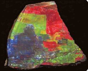
How ammolite gemstones get their vivid colors

Ammolite shows (almost) the complete color spectrum. Credit: Gems & Gemology (2001). DOI: 10.5741/gems.37.1.4

The origins of vivid colors within the gemstone ammolite—a rare type of brightly colored fossilized ammonite shell—are reported in research published in Scientific Reports.

The colors of ammolite occur within a preserved layer of nacre—also known as mother-of-pearl—which consists of layered plates of the mineral aragonite and a small amount of organic material such as proteins. Although it is thought that the colors of ammolite arise from the interaction of light with these layers, the origins of these colors have not been evaluated experimentally.

Hiroaki Imai and colleagues investigated the structural and optical properties of ammolite specimens from Alberta, Canada using electron microscopy and simulations. They then compared these to the properties of paler nacre from an ammonite fossil from Madagascar as well as abalone and nautilus shells.

The authors identified similar structures of stacked aragonite plates within all samples but found that the thickness of these plates and the size of the gaps between them varied.

They found that the brightness of ammolite colors is caused by light reflecting off four nanometer-wide gaps between aragonite plates and by the even distribution of layers of uniform thickness within the nacre.

They suggest that the paler color of nacre in the other samples is caused by larger gaps or a lack of gaps between aragonite plates, the presence of organic material within these gaps, or by variations in the distribution of layers within the nacre.

The authors suggest that their findings could inform the development of non-fading colored paints.

Reference:
Brilliant structural colors originating from reflection by nanogaps of nacreous layers in fossilized ammonite shells, Scientific Reports (2025). DOI: 10.1038/s41598-025-21872-z

Note: The above post is reprinted from materials provided by Nature Publishing Group.

Fossil lichen from Devonian era shows how fungi-algae alliance paved way for terrestrial life

Credit: J. Lacerda
Credit: J. Lacerda

Lichens were already widespread more than 410 million years ago, according to a new international study that identifies a fossil from Brazil as one of the oldest lichen in Earth’s history.

The team used cutting-edge X-ray imaging and other modern techniques to examine a fossil known as Spongiophyton, from the Devonian time period (about 419.2 to 358.9 million years ago).

The study brought together more than 20 institutions and advanced facilities in Brazil, Australia, the U.S., the U.K., and France. The results are published in Science Advances.

According to lead author Dr. Bruno Becker-Kerber from Harvard University, the fossil shows a similar combination of fungi and algae to modern lichens. “Our findings show that lichens were not marginal organisms, but key pioneers in the transformation of Earth’s surface,” he said. “They helped create the soil that allowed plants and animals to take hold and diversify on land.”

The results suggest ancient lichens first evolved in the cold polar regions of the supercontinent Gondwana, in areas that correspond to modern-day South America and Africa.

“Spongiophyton is an extraordinary fossil with extraordinary preservation. It is essentially mummified with organic matter intact,” ANU Professor Jochen Brocks said. “The tough material in simple plants is cellulose. Lichens, on the other hand, are decidedly weird—they are composed of the same material that makes beetles and other insects tough—chitin.

“Chitin is loaded with the element nitrogen. When we analyzed Spongiophyton, we got an enormous nitrogen signal, never seen before. You rarely get such a clear result, it was a Eureka moment.”

According to the authors, lichens still play a crucial role today in producing soil, recycling nutrients, and capturing carbon in extreme environments from deserts to polar regions. Yet their origins have remained obscure due to their fragile nature and scarce fossil record.

“This work shows how essential it is to combine conventional methodologies with cutting-edge techniques,” co-author Nathaly L. Archilha from the Brazilian Synchrotron Light Laboratory said. “Initial measurements guided us toward key regions of interest, and only then could we collect 3D nanometric imaging, revealing the complex fungal and algal networks that define Spongiophyton as a true lichen.”

Reference:
Bruno Becker-Kerber et al, The rise of lichens during the colonization of terrestrial environments, Science Advances (2025). DOI: 10.1126/sciadv.adw7879

Note: The above post is reprinted from materials provided by The Australian National University.

Oldest known 3D burrow systems uncovered in Hubei’s Shibantan biota

Treptichnus in the Shibantan assemblage in the Wuhe area. Credit: NIGPAS

A research team from the Nanjing Institute of Geology and Paleontology of the Chinese Academy of Sciences (NIGPAS) has made progress in studying the Shibantan biota in Yichang, Hubei Province, uncovering the oldest known complex three-dimensional burrow systems to date. Preserved in approximately 550-million-year-old strata, these trace fossils show that complex animal behaviors were modifying the seafloor environment nearly 10 million years earlier than previously thought.

The work appears in Science Advances.

The Ediacaran–Cambrian transition, around 539 million years ago, marks one of the most significant ecosystem revolutions in Earth’s history. A key driver of this ecological shift was the transition of metazoan behavior from simple two-dimensional surface activities to three-dimensional exploration deep into sediments.

This “substrate revolution” transformed the seafloor from a uniform, matground-dominated system into a heterogeneously, bioturbated modern-style seabed, permanently altering the trajectory of Earth’s environmental and biological evolution.

The researchers conducted a systematic study of trace fossils from the Shibantan biota (approximately 550–543 million years old). They identified multiple ichnospecies within the genus Treptichnus and established a new ichnospecies, Treptichnus streptosus. By combining these findings with previously discovered three-dimensional trace fossils such as Lamonte and tadpole-shaped traces from the same biota, the study offers an in-depth analysis of the evolutionary and ecological significance of the emergence of animals’ vertical exploration behavior.

The findings reveal that complex animal behaviors emerged on the eve of the Cambrian explosion.

Treptichnus is a landmark trace fossil, representing the first 3D exploration of sediments by animals, and holds importance in evolutionary biology, animal behavior, and ecology.

The first appearance of T. pedum, a member of this genus, formally defines the Ediacaran–Cambrian boundary. The new discovery from the Shibantan biota predates this revolutionary behavior. In addition to reporting the new species T. streptosus, the study identifies other ichnospecies including T. cf. bifurcus, T. rectangularis, and T. pollardi, demonstrating that animal burrowing behaviors had already achieved considerable diversity by this period.

Furthermore, the Shibantan biota preserves other three-dimensional burrows, such as Lamonte and tadpole-shaped traces. The concentrated occurrence of these vertical exploration behaviors reflects early sedimentary ecological stratification and complex foraging strategies, indicating a gradually enhanced ability of trace-making organisms to engineer substrates.

The study found that Lamonte caused intensive bioturbation within the Shibantan biota. This not only disrupted microbial mats on the sediment surface but also dismantled the ecological environment of Ediacara-type organisms that depended on these mats. This suggests bioturbation may have been a contributing factor to the first extinction event of the Ediacara biota around 550 million years ago.

The emergence of these complex behaviors and their cumulative ecological effects intensified toward the end of the Ediacaran Period. This led to the gradual decline of microbial mats, continuously eroding the ecological foundation of Ediacara-type organisms while creating new ecological opportunities for the diversification of other metazoans. Driven by the synergy of various biological and non-biological factors, this process ultimately contributed to the profound ecosystem transformation during the Ediacaran–Cambrian transition.

This research further confirms that the rich and diverse assemblage of trace fossils and body fossils preserved in the Shibantan biota provides a window for studying major ecosystem changes at the transition between the Precambrian and Phanerozoic eons.

Reference:
Science Advances (2025). DOI: 10.1126/sciadv.adx9449

Note: The above post is reprinted from materials provided by Chinese Academy of Sciences.

Rare fossil find reveals early evolution of mosquitoes

Credit: André Amaral, AG Haug

In amber some 99 million years old, LMU researchers have discovered the oldest known mosquito larva. The Cretaceous fossil comes from the Kachin region in Myanmar and was preserved in excellent condition. Described as a new species of a new genus, it has been given the name Cretosabethes primaevus. It represents both the first mosquito larva preserved in amber and the first immature mosquito from the Mesozoic Era, as only the fossils of adult mosquitoes from this era had previously been found.

More remarkable still is the morphology of the insect: “This fossil is unique, because the larva is very similar to modern species—in contrast to all other fossil discoveries of mosquitoes from this period, which exhibit highly unusual morphological traits that are no longer present in today’s species,” says zoologist André Amaral, lead author of the study published in Gondwana Research and doctoral researcher in Professor Joachim Haug’s team at LMU’s Faculty of Biology.

These oldest known mosquito fossils come from adult insects and were also found in amber deposits about 99 million years old. Due to their morphology, which differs sharply from that of modern species, they are interpreted as representing a distinct group, Burmaculicinae, an extinct lineage within the mosquito group (Culicidae). Cretosabethes primaevus, by contrast, belongs to the Sabethini group, which includes extant species.

The evolutionary origins of mosquitoes have been situated in the Jurassic period about 201–145 million years ago, based on the fossils that have been found to date. Estimates based on molecular phylogenies widely diverge and yield results between the Triassic and the Jurassic.

The discovery by the LMU researchers provides new clues: “Our results provide strong indications that mosquitoes had already diversified in the Jurassic period and that the morphology of their larvae has remained remarkably similar for almost 100 million years,” says Amaral. This calls into question previous assumptions about the early evolution of this insect group, he observes, and affords new insights into its evolutionary ecology.

Like the larvae of extant species from the Sabethini group, the larva of Cretosabethes primaevus is thus thought to have lived in small accumulations of water, such as form in hollows in tree branches or between the leaves of epiphytic plants. For a drop of resin to fall into such a tiny pool of water and preserve an aquatic larva in amber is most unlikely and therefore the discovery is a rare stroke of luck.

Most amber fossils come from terrestrial or flying creatures that lived on or near resin-producing trees. The most common groups of arthropods discovered in Myanmar amber are spiders, beetles, hymenopterans (bees, wasps, and ants), and true bugs (Hemiptera) as well as adult flies (Diptera).

Reference:
André P. Amaral et al, First fossil mosquito larva in 99-million-year-old amber with a modern type of morphology sheds light on the evolutionary history of mosquitoes (Diptera: Culicidae), Gondwana Research (2025). DOI: 10.1016/j.gr.2025.09.011

Note: The above post is reprinted from materials provided by Ludwig Maximilian University of Munich.

An old fish fossil tells a new story about lamniform shark evolution

On the left, one of the gigantic cardabiodontid fossils (NTM P22-33) with a diameter of 12.5 cm (courtesy of Dr. Mohamed Bazzi); on the right, anterior or posterior, dorsal, anterior, and dorsal fossils from a 5-meter-long (16.4 feet) adult Great White shark, Carcharodon carcharias (LACM I-35875-1). Credit: Mike Newbrey

An international, multi-university research team, including scientists from Columbus State University, has unearthed a crucial new piece of the puzzle in the evolution of sharks.

A recent study published in Communications Biology, “Early gigantic lamniform marks the onset of mega-body size in modern shark evolution,” has identified a new, extinct lamniform shark—a group that includes modern-day great white and mako sharks. It marks the earliest known example of a gigantic shark, suggesting that the trend of mega-body size in modern shark evolution began much earlier than previously thought.

The team, led by Dr. Mohamad Bazzi of Stanford University, included Dr. Mike Newbrey of Columbus State’s Department of Biology and 2020 alumna Tatianna Blake. They derived their conclusions after studying specimens from the Darwin Formation that outcrops at Darwin, Australia. These specimens, collected by other researchers in the 1980s, had been stored in a museum collection and remained unstudied until recently, when the team examined them in detail.

By analyzing newly discovered fossil evidence, the group’s conclusions rewrite the timeline of the evolution of megabody-sized sharks as apex predators, pushing it back by 15 million years. The 115-million-year-old fossil vertebrae were used to estimate a body length of 6 meters to 8 meters (19.5 feet to 26.3 feet), and a weight of over 3 tons. The earliest lamniform fossils were small and uncontestably date back to about 135 million years old.

“As a field, we are curious about the environmental and ecological conditions needed to evolve mega-body size,” Newbrey explained. “As researchers, we need a rigorous method of estimating body size to answer the question about the conditions needed to evolve large body sizes in lamniform sharks.”

Newbrey went on to explain that the size estimates used in this study were derived from a novelly compiled and analyzed dataset of vertebrae from 10 species of living lamniform sharks with known body lengths. Prior to this study, there was no way to cross-evaluate the effects of different species on body-length estimates from fossil material, nor was there an informed interpretation of body-length estimates from incomplete fossil material of lamniform sharks.

Previous interpretations suggested that gigantic lamniform sharks evolved in the Late Cretaceous period (100.5 to 66 million years ago) with a specialization in pelagic lifestyles. However, Newbrey said the team’s investigation supports an earlier evolution of gigantic lamniform sharks in the Early Cretaceous period (145.1 to 100.5 million years ago) during a time when it was relatively cooler than the Late Cretaceous period. As a result of this research, the field has a new set of questions to consider regarding the evolution of gigantic lamniform sharks.

From student to published researcher

In addition to the team’s discovery, the project uncovered another one—Columbus State undergrad Tatianna Blake’s interest in research. Newbrey mentored Blake as part of her undergraduate research project, which she completed as a biology student. Her involvement in Newbrey’s line of research continued after she graduated, which landed her a co-authorship credit in Communications Biology.

“[T]hat opportunity [to work with Newbrey] alone had a lasting impact on my academic trajectory,” Blake recalled. “The structure of my undergraduate program—which required students to engage in faculty-led research—was instrumental in exposing me to research in the first place. The mentorship I received [from Newbrey] and the hands-on nature of the project itself provided the foundation I needed to appreciate and pursue research further.”

Continuing scientific research wasn’t necessarily on Blake’s radar after she graduated with her biology degree and concentration in pre-veterinary medicine. She instead applied her minor in military and advanced leadership to serve as a U.S. Army logistics officer, and later, teaching high school aquatic science and astronomy. Blake is now focused on being accepted to a doctoral program and conducting research in marine science.

“[Dr. Newbrey’s] passion for ichthyology inspired me to explore fish research myself,” she said of her experience as an undergraduate researcher. “The project, which focused on a lesser-known fossil fish species, quickly captured my interest. It was exciting to work with actual fossil specimens and contribute original data to a field I hadn’t previously considered. That experience sparked a deeper appreciation for research and its broader impact.”

Newbrey said not every project leads to publication in such a prestigious scientific journal, but including students in faculty-led research is a priority for him and his faculty colleagues.

“Students perform best academically, and later professionally, when they have opportunities to apply what they learn by doing,” he said.

“We strive to include our students in research opportunities early in their studies, so they can realize the power and potential of how what they learn in the classroom contributes to the science and education fields, while also bettering the communities in which we live.”

Future research applications

Newbrey said this new analysis will be useful for many future studies of lamniform sharks. The new large lamniform predates other giant sharks, and this study provides a protocol to estimate body size for the study of the effects of the environmental and ecological factors that allowed sharks to reach such colossal proportions.

“For example, the team notes that the large cardabiodontid existed during a relatively cold time, and they speculate that large body size may have enabled these particular sharks to survive in colder waters, thereby capitalizing on a vacant niche filled today by other large lamniform sharks,” he said.

“Being able to estimate body size from isolated vertebral material will enable us to answer larger questions about shark evolution while considering the effects of climatic change.”

Reference:
Mohamad Bazzi et al, Early gigantic lamniform marks the onset of mega-body size in modern shark evolution, Communications Biology (2025). DOI: 10.1038/s42003-025-08930-y

Note: The above post is reprinted from materials provided by Columbus State University.

How diamonds reach the surface

Diamond
Diamond

If you’ve ever held or beheld a diamond, there’s a good chance it came from a kimberlite. Over 70% of the world’s diamonds are mined from these unique volcanic structures. Yet despite decades of study, scientists are still working to understand how exactly kimberlites erupt from deep in Earth’s mantle to the surface.

Kimberlites — carrot-shaped volcanic pipes that erupt from mantle depths greater than 150 km — have long fascinated geologists as windows into the deep Earth. Their mantle-derived melt ascends rapidly through the mantle and crust, with some estimates suggesting ascent rates of up to 80 miles per hour before kimberlites erupt violently at the surface. Along the way, the magma captures xenoliths and xenocrysts, fragments of the rocks encountered on its path.

“They’re very interesting and still very enigmatic rocks,” despite being well-studied, says Ana Anzulović, a doctoral research fellow at the University of Oslo’s Centre for Planetary Habitability.

In a study published this month in the journal Geology, Anzulović and colleagues from the University of Oslo have taken a major step toward solving the puzzle. By modelling how volatile compounds like carbon dioxide and water influence the buoyancy of proto-kimberlite melt relative to surrounding materials, they quantified for the first time what it takes to erupt a kimberlite.

Diamonds make it to the surface in kimberlites because their rapid ascent prevents them from reverting to graphite, which is more stable at shallow pressures and temperatures. But the composition of the kimberlite’s original melt — and how it rises so fast — has remained mysterious.

“They start off as something that we cannot measure directly,” says Anzulović. “So we don’t know what a proto-kimberlite, or parental, melt would be like. We know approximately but everything we know basically comes from the very altered rocks that get emplaced.”

To constrain the composition of these parental melts, the team focused on the Jericho kimberlite, which erupted into the Slave craton of far northwest Canada. Using chemical modelling, they tested different original mixtures of carbon dioxide and water.

“Our idea was, well, let’s try to create a chemical model of a kimberlite, then vary CO2 and H2O,” says Anzulović. “Think of it as trying to sample a kimberlite as it ascends at different pressure and temperature points.”

The researchers used molecular dynamics software to simulate atomic forces and track how atoms in a kimberlite melt move under varying depths. From these calculations, they determined the density of the melt at different conditions and whether it remained buoyant enough to rise.

“The most important takeaway from this study is that we managed to constrain the amount of CO2 that you need in the Jericho kimberlite to successfully ascend through the Slave craton,” Anzulović says. “Our most volatile-rich composition can carry up to 44% of mantle peridotite, for example, to the surface, which is really an impressive number for such a low viscosity melt.”

The study also shows how volatiles play distinct roles. Water increases diffusivity, keeping the melt fluid and mobile. Carbon dioxide helps structure the melt at high pressures but, near the surface, it degasses and drives the eruption upward. For the first time, researchers demonstrated that the Jericho kimberlite needs at least 8.2% CO2 to erupt; without it, diamonds would remain locked in the mantle.

“I was actually pretty surprised that I can take such a small scale system and actually observe, ‘Okay, if I don’t put any carbon in, this melt will be denser than the craton, so this will not erupt,'” says Anzulović. “It’s great that modeling kimberlite chemistry can have implications for such a large-scale process.”

Reference:
Ana Anzulović, Anne H. Davis, Carmen Gaina, Razvan Caracas. Buoyancy of volatile-rich kimberlite melts, magma ascent, and xenolith transport. Geology, 2025; DOI: 10.1130/G53387.1

Note: The above post is reprinted from materials provided by Geological Society of America.

Dinosaurs were thriving when the asteroid struck

Artist illustration of an alamosaurus. (Credit: Natalia Jagielska)

For much of the past century, scientists thought dinosaurs were already in decline long before the asteroid impact that ended their reign 66 million years ago. However, a new study published in Science by researchers from Baylor University, New Mexico State University, The Smithsonian Institution, and several international partners challenges that long-standing belief.

The findings reveal that dinosaurs were not fading away at all — they were thriving.

A final flourish in the San Juan Basin

In northwestern New Mexico, layers of ancient rock hold clues to a lively, previously overlooked chapter of Earth’s history. Within the Naashoibito Member of the Kirtland Formation, scientists found evidence of rich dinosaur ecosystems that continued to flourish until just before the asteroid struck.

High-precision dating determined that fossils from these rocks are between 66.4 and 66 million years old, placing them right at the boundary between the Cretaceous and Paleogene periods, when the global extinction event occurred.

“The Naashoibito dinosaurs lived at the same time as the famous Hell Creek species in Montana and the Dakotas,” said Daniel Peppe, Ph.D., associate professor of geosciences at Baylor University. “They were not in decline — these were vibrant, diverse communities.”

Dinosaurs in their prime

The fossil evidence from New Mexico tells a strikingly different story from what many had assumed. Instead of dwindling, dinosaurs across North America were thriving in distinct regional communities. By analyzing ecological and geographic patterns, researchers found that dinosaur populations in western North America were divided into separate “bioprovinces” shaped primarily by regional temperature differences rather than by mountains or rivers.

“What our new research shows is that dinosaurs are not on their way out going into the mass extinction,” said first author Andrew Flynn, Ph.D. ’20, assistant professor of geological sciences at New Mexico State University. “They’re doing great, they’re thriving and that the asteroid impact seems to knock them out. This counters a long-held idea that there was this long-term decline in dinosaur diversity leading up to the mass extinction making them more prone to extinction.”

Life after impact

The asteroid impact brought the age of dinosaurs to an abrupt end, but the ecosystems they left behind became the foundation for a new evolutionary chapter. Within just 300,000 years, mammals began rapidly diversifying, developing new diets, sizes, and ecological roles.

The same temperature-related patterns that once defined dinosaur ecosystems continued into the Paleocene epoch, guiding how life recovered after the disaster.

“The surviving mammals still retain the same north and south bio provinces,” Flynn said. “Mammals in the north and the south are very different from each other, which is different than other mass extinctions where it seems to be much more uniform.”

Why this discovery matters

This discovery offers more than just a look into the distant past. It underscores both the resilience and fragility of life on Earth. Conducted on public lands managed by the U.S. Bureau of Land Management, the research highlights how protected landscapes can unlock vital insights into how ecosystems respond to global upheaval.

By refining the timeline of the dinosaurs’ final days, the study reveals that their extinction was not a slow decline but an abrupt, catastrophic end to a flourishing era of life — cut short by chance from beyond the sky.

About the authors

In addition to Peppe and Flynn, the research team included scientists from Baylor University, New Mexico State University, the Smithsonian Institution, the University of Edinburgh, University College London and multiple U.S. and international institutions.

  • Stephen L. Brusatte, Ph.D., The University of Edinburgh
  • Alfio Alessandro Chiarenza, Ph.D., Royal Society Newton International Fellow, University College London
  • Jorge Garcia-Giron, Ph.D., University of Leon
  • Adam J. Davis, Ph.D., WSP USA Inc.
  • C. Will Fenley, Ph.D., Valle Exploration
  • Caitlin E. Leslie, Ph.D., ExxonMobil
  • Ross Secord, Ph.D., University of Nebraska-Lincoln
  • Sarah Shelley, Ph.D., Carnegie Museum of Natural History
  • Anne Weil, Ph.D., Oklahoma State University
  • Matthew T. Heizler, Ph.D., New Mexico Institute of Mining and Technology
  • Thomas E. Williamson, Ph.D., New Mexico Museum of Natural History and Science

Funding

This research was supported by the National Science Foundation, European Research Council, Royal Newton International Fellowship, Geologic Society of America Graduate Research Grant, Baylor University James Dixon Undergraduate Fieldwork Fellowship (AGF), the European Union Next Generation, the British Ecological Society and the American Chemical Society — Petroleum Research Fund.

The researchers would like to thank the Bureau of Land Managementfor providing collecting permits and supporting the research.

Reference:
Andrew G. Flynn, Stephen L. Brusatte, Alfio Alessandro Chiarenza, Jorge García-Girón, Adam J. Davis, C. Will Fenley, Caitlin E. Leslie, Ross Secord, Sarah Shelley, Anne Weil, Matthew T. Heizler, Thomas E. Williamson, Daniel J. Peppe. Late-surviving New Mexican dinosaurs illuminate high end-Cretaceous diversity and provinciality. Science, 2025; 390 (6771): 400 DOI: 10.1126/science.adw3282

Note: The above post is reprinted from materials provided by Baylor University.

Scientists just cracked a 60-million-year-old volcanic mystery

The progression of the 2021 Fagradalsfjall eruption.

What do the rumblings of Iceland’s volcanoes have in common with the now peaceful volcanic islands off Scotland’s western coast and the spectacular basalt columns of the Giant’s Causeway in Northern Ireland?

About sixty million years ago, the Icelandic mantle plume — a fountain of hot rock that rises from Earth’s core-mantle boundary — unleashed volcanic activity across a vast area of the North Atlantic, extending from Scotland and Ireland to Greenland.

For decades, scientists have puzzled over why this burst of volcanism was so extensive. Now, research led by the University of Cambridge has found that differences in the thickness of tectonic plates around the North Atlantic might explain the widespread volcanism.

The researchers compiled seismic and temperature maps of Earth’s interior, finding that patches of thinner tectonic plate acted like conduits, funneling the plume’s molten rock over a wide area.

Iceland, which is one of the most volcanically active places on Earth, owes its origin largely to the mantle plume. Beyond volcanism, the Iceland Plume’s influence even extends to shaping the seafloor and ocean circulation in the North Atlantic and, in turn, climate through time. Despite its global significance, many aspects of the plume’s behavior and history remain elusive.

“Scientists have a lot of unanswered questions about the Iceland plume,” said Raffaele Bonadio, a geophysicist at Cambridge’s Department of Earth Sciences and lead author of the study.

Bonadio set out to explain why the plume’s volcanic imprint was much more widespread sixty million years ago — before the Atlantic opened — forming volcanoes and lava outpourings stretching over thousands of kilometers. The pattern could be explained by the mantle plume spreading outward in a branched, flowing formation, Bonadio explained, “but evidence for such flow has been scarce.”

In search of answers, Bonadio focused on a segment of the North Atlantic Igneous Province to better understand the complex distribution of volcanoes in Scotland and Ireland. He wanted to know if the structure of Earth’s tectonic plates played a role in the surface expression of volcanism.

Using seismic data extracted from earthquakes, Bonadio created a computer-generated image of Earth’s interior beneath Britain and Ireland. This method, known as seismic tomography, works similarly to a medical CT scan, revealing hidden structures deep within the planet. Bonadio coupled this with seismic thermography measurements — a new method developed by the team — which reveal variations in the temperature and thickness of the tectonic plate.

He found that northwest Scotland and Ireland’s volcanoes formed in areas where the lithosphere (Earth’s rigid outer layer that makes up the tectonic plates) is thinner and weaker.

“We see ancient volcanoes concentrated within this corridor of thin lithosphere beneath the Irish Sea and surrounding areas,” said Bonadio. He thinks the hot plume material was preferentially funneled along this corridor, ponding in the thin plate areas due to its buoyancy.

Previously, some scientists had put forward alternative, non-mantle plume origins for the volcanic activity, said Bonadio. But his new research shows the scattering could be explained by the magma being diverted and re-routed to areas of thinner lithosphere.

Sergei Lebedev, from the University of Cambridge said, “this striking correlation suggests that hot plume material eroded the lithosphere in this region. This resulting combination of thin lithosphere, hot asthenosphere and decompression melting likely caused the uplift and volcanic activity.”

Previously, the authors have found a close link between the uneven distribution of earthquakes in Britain and Ireland and the thickness of the lithosphere, showing how the scars left by the mantle plume influence seismic hazards today.

Bonadio and Lebedev are also using their methods to map geothermal energy resource potential. “In Britain and Ireland, the greatest supply of heat from the Earth’s mantle is in the same places where volcanoes erupted sixty million years ago, and where the lithosphere is thinner,” said Lebedev. He and Bonadio are working with international colleagues to apply their new seismic thermography methods to global geothermal assessment.

Reference:
Raffaele Bonadio, Sergei Lebedev, David Chew, Yihe Xu, Javier Fullea, Thomas Meier. Volcanism and long-term seismicity controlled by plume-induced plate thinning. Nature Communications, 2025; 16 (1) DOI: 10.1038/s41467-025-62967-5

Note: The above post is reprinted from materials provided by University of Cambridge.

MOST POPULAR

MORE ARTICLES