A remarkable new species of horned dinosaur has been unearthed in Grand Staircase-Escalante National Monument, southern Utah. The huge plant-eater inhabited Laramidia, a landmass formed when a shallow sea flooded the central region of North America, isolating western and eastern portions for millions of years during the Late Cretaceous Period.
The newly discovered dinosaur, belonging to the same family as the famous Triceratops, was announced today in the British scientific journal, Proceedings of the Royal Society B.
The study, funded in large part by the Bureau of Land Management and the National Science Foundation, was led by Scott Sampson, when he was the Chief Curator at the Natural History Museum of Utah at the University of Utah. Sampson is now the Vice President of Research and Collections at the Denver Museum of Nature & Science.
Additional authors include Eric Lund (Ohio University; previously a University of Utah graduate student), Mark Loewen (Natural History Museum of Utah and Dept. of Geology and Geophysics, University of Utah), Andrew Farke (Raymond Alf Museum), and Katherine Clayton (Natural History Museum of Utah).
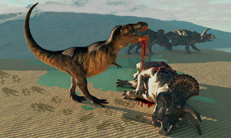
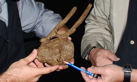
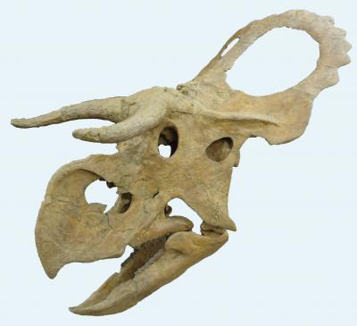
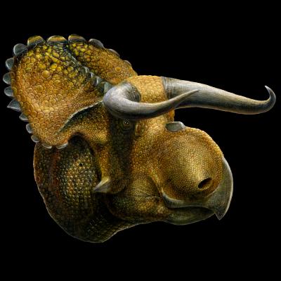
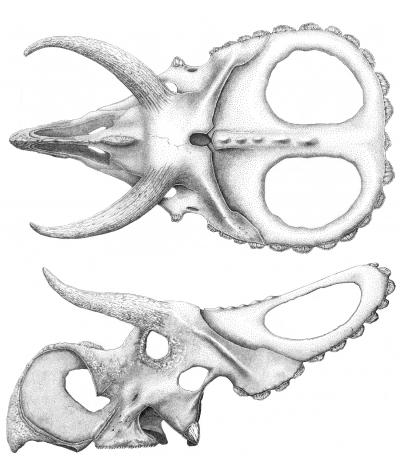
Horned dinosaurs, or “ceratopsids,” were a group of big-bodied, four-footed herbivores that lived during the Late Cretaceous Period. As epitomized by Triceratops, most members of this group have huge skulls bearing a single horn over the nose, one horn over each eye, and an elongate, bony frill at the rear. The newly discovered species, Nasutoceratops titusi, possesses several unique features, including an oversized nose relative to other members of the family, and exceptionally long, curving, forward-oriented horns over the eyes.
The bony frill, rather than possessing elaborate ornamentations such as hooks or spikes, is relatively unadorned, with a simple, scalloped margin. Nasutoceratops translates as “big-nose horned face,” and the second part of the name honors Alan Titus, Monument Paleontologist at Grand Staircase-Escalante National Monument, for his years of research collaboration.
For reasons that have remained obscure, all ceratopsids have greatly enlarged nose regions at the front of the face. Nasutoceratops stands out from its relatives, however, in taking this nose expansion to an even greater extreme. Scott Sampson, the study’s lead author, stated, “The jumbo-sized schnoz of Nasutoceratops likely had nothing to do with a heightened sense of smell — since olfactory receptors occur further back in the head, adjacent to the brain — and the function of this bizarre feature remains uncertain.”
Paleontologists have long speculated about the function of horns and frills on horned dinosaurs. Ideas have
ranged from predator defense and controlling body temperature to recognizing members of the same species. Yet the dominant hypothesis today focuses on competing for mates—that is, intimidating members of the same sex and attracting members of the opposite sex. Peacock tails and deer antlers are modern examples. In keeping with this view, Mark Loewen, a co-author of the study claimed that, “The amazing horns of Nasutoceratops were most likely used as visual signals of dominance and, when that wasn’t enough, as weapons for combatting rivals.”
A Treasure Trove of Dinosaurs on the Lost Continent of Laramidia
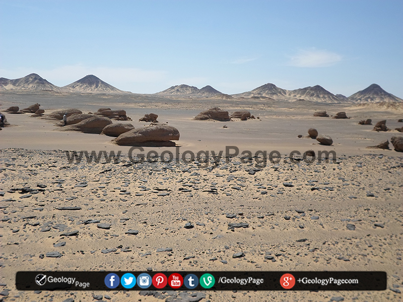
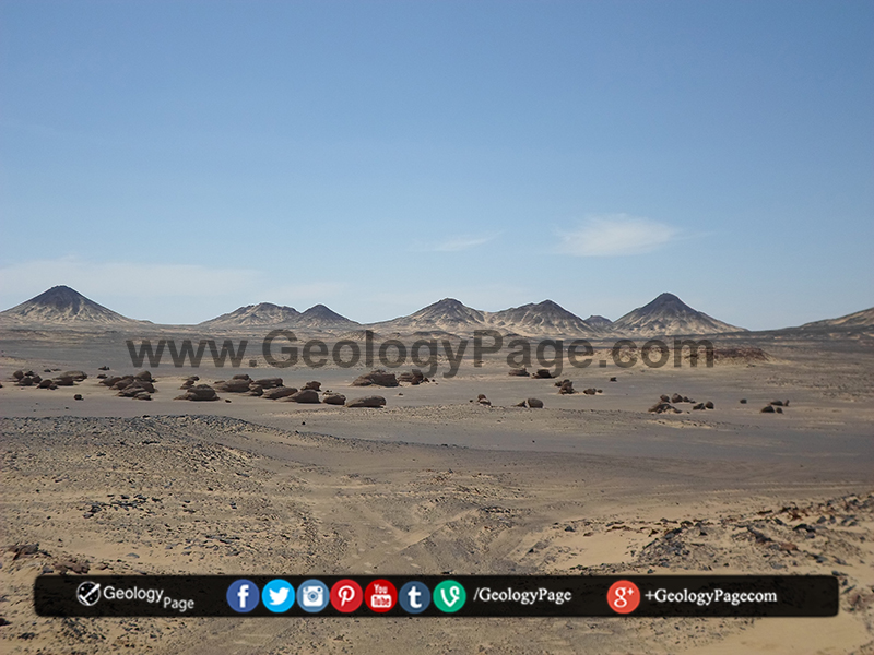
Nasutoceratops was discovered in Grand Staircase-Escalante National Monument (GSENM), which encompasses 1.9 million acres of high desert terrain in south-central Utah. This vast and rugged region, part of the National Landscape Conservation System administered by the Bureau of Land Management, was the last major area in the lower 48 states to be formally mapped by cartographers. Today GSENM is the largest national monument in the United States. Sampson proclaimed that, “Grand Staircase-Escalante National Monument is the last great, largely unexplored dinosaur boneyard in the lower 48 states.”
For most of the Late Cretaceous, exceptionally high sea levels flooded the low-lying portions of several continents around the world. In North America, a warm, shallow sea called the Western Interior Seaway extended from the Arctic Ocean to the Gulf of Mexico, subdividing the continent into eastern and western landmasses, known as Appalachia and Laramidia, respectively. Whereas little is known of the plants and animals that lived on Appalachia, the rocks of Laramidia exposed in the Western Interior of North America have generated a plethora of dinosaur remains. Laramidia was less than one-third the size of present day North America, approximating the area of Australia.
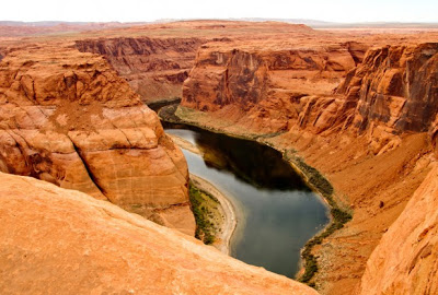
Most known Laramidian dinosaurs were concentrated in a narrow belt of plains sandwiched between the seaway to the east and mountains to the west. Today, thanks to an abundant fossil record and more than a century of collecting by paleontologists, Laramidia is the best known major landmass for the entire Age of Dinosaurs, with dig sites spanning from Alaska to Mexico. Utah was located in the southern part of Laramidia, which has yielded far fewer dinosaur remains than the fossil-rich north. The world of dinosaurs was much warmer than the present day; Nasutoceratops lived in a subtropical swampy environment about 100 km from the seaway.
Beginning in the 1960’s, paleontologists began to notice that the same major groups of dinosaurs seemed to be present all over this Late Cretaceous landmass, but different species of these groups occurred in the north (for example, Alberta and Montana) than in the south (New Mexico and Texas). This finding of “dinosaur provincialism” was very puzzling, given the giant body sizes of many of the dinosaurs together with the diminutive dimensions of Laramidia. Currently, there are five giant (rhino-to-elephant-sized) mammals on the entire continent of Africa. Seventy-six million years ago, there may have been more than two dozen giant dinosaurs living on a landmass about one-quarter that size. Co-author Mark Loewen noted that, “We’re still working to figure out how so many different kinds of giant animals managed to co-exist on such a small landmass?” The new fossils from GSENM are helping us explore the range of possible answers, and even rule out some alternatives.
During the past dozen years, crews from the Natural History Museum of Utah, the Denver Museum of Nature & Science and several other partner institutions (e.g., the Utah Geologic Survey, the Raymond Alf Museum of Paleontology, and the Bureau of Land Management) have unearthed a new assemblage of more than a dozen dinosaurs in GSENM. In addition to Nasutoceratops, the collection includes a variety of other plant-eating dinosaurs—among them duck-billed hadrosaurs, armored ankylosaurs, dome-headed pachycephalosaurs, and two other horned dinosaurs, Utahceratops and Kosmoceratops — together with carnivorous dinosaurs great and small, from “raptor-like” predators to a mega-sized tyrannosaur named Teratophoneus. Amongst the other fossil discoveries are fossil plants, insect traces, clams, fishes, amphibians, lizards, turtles, crocodiles, and mammals. Together, this diverse bounty of fossils is offering one of the most comprehensive glimpses into a Mesozoic ecosystem. Remarkably, virtually all of the identifiable dinosaur remains found in GSENM belong to new species, providing strong support for the dinosaur provincialism hypothesis.
Andrew Farke, a study co-author, noted that, “Nasutoceratops is one of a recent landslide of ceratopsid discoveries, which together have established these giant plant-eaters as the most diverse dinosaur group on Laramidia.”
Eric Lund, another co-author as well as the discoverer of the new species, stated that, “Nasutoceratops is a wondrous example of just how much more we have to learn about with world of dinosaurs. Many more exciting fossils await discovery in Grand Staircase-Escalante National Monument.”
Fact Sheet: Major Points of the Paper
(1) A remarkable new horned dinosaurs Nasutoceratops titusi, has been unearthed in Grand Staircase-Escalante National Monument, southern Utah.
(2) Nasutoceratops is distinguished by a number of unique features, including an oversized nose and elongate, forward-curving horns over the eyes.
(3) This animal lived in a swampy, subtropical setting on the “island continent” of western North America, also known as “Laramidia.”
(4) Nasutoceratops appears to belong to a previously unrecognized group of horned dinosaurs that lived on Laramidia, and provides strong evidence supporting the idea that distinct northern and southern dinosaur communities lived on this landmass for over a million years during the Late Cretaceous.
New Dinosaur Name: Nasutoceratops titusi.
- The first part of the name, Nasutoceratops, can be translated as the “big-nosed horned face,” in reference to the oversized nose of this plant-eating dinosaur. The second part of the name honors Alan Titus, Monument Paleontologist at Grand Staircase-Escalante National Monument, for all of his work in support of paleontological research in GSENM.
Size
Nasutoceratops was about 15 feet (5 meters) long and 2.5 tonnes.
Relationships
Nasutoceratops belongs to a group of big-bodied horned dinosaurs called “ceratopsids,” the same family as the famous Triceratops. More specifically, they are members of the subset of ceratopsids known as “centrosaurines,” with Avaceratops being the closest known relative within this smaller subset of horned dinosaurs.
Anatomy
- Nasutoceratops was a four-legged (quadrupedal) herbivore.
- Like most other horned dinosaurs, Nasutoceratops had a large horn above each eye, although they are particularly elongate in this animal and forward facing, which is unusual. Rather than a large horn over the nose and an elaborately ornamented frill, both typical of centrosaurines, Nasutoceratops possessed a low, narrow, blade-like horn above the nose and relatively simple frill lacking well developed ornaments.
Age and Geography
- Nasutoceratops lived during the Campanian stage of the Late Cretaceous period, which spanned from approximately 84 million to 70 million years ago. This animal lived about 76 million years ago.
- During the Late Cretaceous, the North American continent was split in two by the Western Interior Seaway. Western North America formed an island continent called Laramidia, stretching from Mexico in the south to Alaska in the north.
- Nasutoceratops lived in Utah at the same time that other, closely related horned dinosaurs lived in Alberta. This finding strong evidence of dinosaur provincialism on Laramidia—that is, the formation of northern and southern dinosaur assemblages during a part of the Late Cretaceous.
Discovery
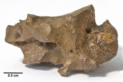
- Nasutoceratops was found in a geologic unit known as the Kaiparowits Formation, abundantly exposed in GSENM, southern Utah.
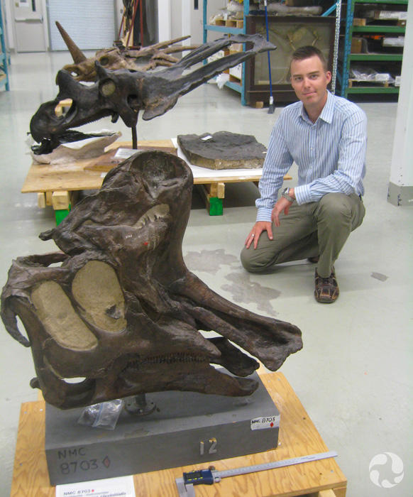
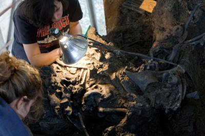
- Nasutoceratops was first discovered by (then) University of Utah masters student Eric Lund in 2006. Additional specimens of this animal were found in subsequent years.
- Nasutoceratops specimens are permanently housed in the collections and on public display at the Natural History Museum of Utah in Salt Lake City, Utah.
- These discoveries are the result of a continuing collaboration between the Natural History Museum of Utah, the Denver Museum of Nature & Science, and the Bureau of Land Management.
Other
- The fossil record of ceratopsid dinosaurs from the southern part of Laramidia has been very poorly known. The discovery of this new dinosaur in Utah helps to fill a major gap in our knowledge.
- Nasutoceratops is part of a previously unknown assemblage dinosaurs discovered in GSENM over the past 12 years.
- The skull of Nasutoceratops is on permanent display at the Natural History Museum of Utah.
- The Bureau of Land Management manages more land—253 million acres—than any other federal agency, and manages paleontological resources using scientific principles and expertise.
- In addition to serving as the Vice President of Research and Collections at the Denver Museum of Nature & Science, the paper’s lead author, Scott Sampson, is also the science advisor and on-air host of the hit PBS KIDS television series, Dinosaur Train.
Note : The above story is reprinted from materials provided by University of Utah