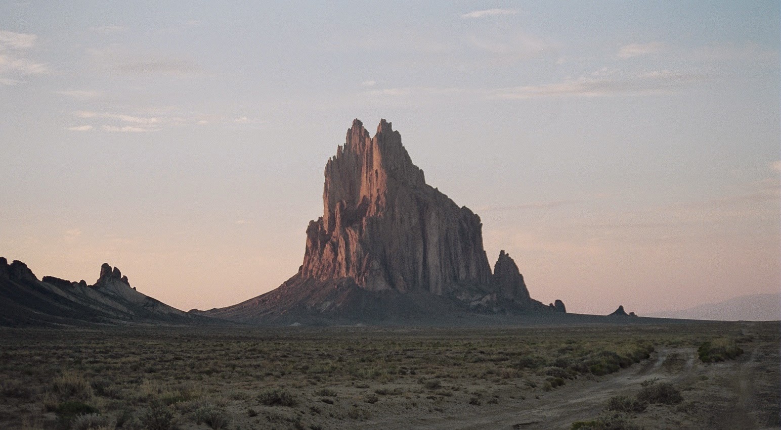
Shiprock, New Mexico, is in the Four Corners region where an atmospheric methane “hot spot” can be seen from space. Researchers are currently in the area, trying to uncover the reasons for the hot spot. Credit: Wikimedia Commons
Researchers from several institutions are in the Four Corners region of the U.S. Southwest with a suite of airborne and ground-based instruments, aiming to uncover reasons for a mysterious methane “hot spot” detected from space.
“With all the ground-based and airborne resources that the different groups are bringing to the region, we have the unique chance to unequivocally solve the Four Corners mystery,” said Christian Frankenberg, a scientist at NASA’s Jet Propulsion Laboratory, Pasadena, California, who is heading NASA’s part of the effort. Other investigators are from the Cooperative Institute for Research in Environmental Sciences (CIRES) in Boulder, Colorado; the National Oceanic and Atmospheric Administration (NOAA); and the University of Michigan, Ann Arbor.
Last fall, researchers including Frankenberg reported that a small region around the Four Corners intersection of Arizona, Colorado, New Mexico and Utah had the highest concentration of methane over background levels of any part of the United States. An instrument on a European Space Agency satellite measuring greenhouse gases showed a persistent atmospheric hot spot in the area between 2003 and 2009. The amount of methane observed by the satellite was much higher than previously estimated.
The satellite observations were not detailed enough to reveal the actual sources of the methane in the Four Corners. Likely candidates include venting from oil and gas activities, which are primarily coalbed methane exploration and extraction in this region; active coal mines; and natural gas seeps.
Researchers from CIRES, NOAA’s Earth Systems Research Laboratory and Michigan are conducting a field campaign called TOPDOWN (Twin Otter Projects Defining Oil Well and Natural gas emissions) 2015, bringing airborne and ground-based instruments to investigate possible sources of the methane hot spot. The JPL team will join the effort on April 17-24. The groups are coordinating their measurements, but each partner agency will deploy its own suite of instruments.
The JPL participants will fly two complementary remote sensing instruments on two Twin Otter research aircraft. The Next-Generation Airborne Visible/Infrared Imaging Spectrometer (AVIRISng), which observes spectra of reflected sunlight, flies at a higher altitude and will be used to map methane at fine resolution over the entire region. Using this information and ground measurements from the other research teams, the Hyperspectral Thermal Emission Spectrometer (HyTES) will fly over suspected methane sources, making additional, highly sensitive measurements of methane. Depending on its flight altitude, the NASA aircraft can image methane features with a spatial resolution better than three feet (one meter) square. In other words, it can create a mosaic showing how methane levels vary every few feet, enabling the identification of individual sources.
With the combined resources, the investigators hope to quantify the region’s overall methane emissions and pinpoint contributions from different sources. They will track changes over the course of the month-long effort and study how meteorology transports emissions through the region.
“If we can verify the methane detected by the satellite and identify its sources, decision-makers will have critical information for any actions they are considering,” said CIRES scientist Gabrielle Pétron, one of the mission’s investigators. Part of President Obama’s recent Climate Action Plan calls for reductions in methane emissions.
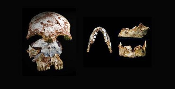
Researchers found an ancient human skull, left, with modern characteristics, and a human jaw, right, with modern and archaic traits, in the same cave in northern Laos. Both artifacts date to 46,000 to 63,000 years ago. Credit: Fabrice Demeter
An ancient human skull and a jawbone found a few meters away in a cave in northern Laos add to the evidence that early modern humans were physically quite diverse, researchers report in PLOS ONE.
The skull, found in 2009 in a cave known as Tam Pa Ling in the Annamite Mountains of present-day Laos, and reported in 2012 in the Proceedings of the National Academy of Sciences, is the oldest modern human fossil found in Southeast Asia. Its discovery pushed back the date of modern human migration through the region by as much as 20,000 years. It revealed that early humans who migrated to the islands and coasts of Southeast Asia after migrating out of Africa also traveled inland much earlier than previously thought, some 46,000 to 63,000 years ago.
The jaw was discovered in late 2010 and is roughly the same age as the skull. Unlike the skull, it has both modern and archaic human traits.
“In addition to being incredibly small in overall size, this jaw has a mixture of traits that combine typical modern human anatomy, such as the presence of a protruding chin, with traits that are more common of our archaic ancestors like Neandertals — for example, very thick bone to hold the molars in place,” said University of Illinois anthropology professor Laura Shackelford, who led the study with anthropologist Fabrice Demeter, of the National Museum of Natural History in Paris.
This combination of archaic and modern human traits is not unusual, Shackelford said. Other ancient human fossils from Africa, Eastern Europe and China also exhibit this amalgam of characteristics, she said.
“Some researchers have used these features as evidence that modern humans migrating into new regions must have interbred with the archaic populations already present in those regions,” Shackelford said. “But a more productive way to look at this variation is to see it as we see people today — showing many traits along a continuum.
“Tam Pa Ling is an exceptional site because it shows that very early modern humans migrating and settling in eastern Asia demonstrated a wide range of anatomy,” Shackelford said.
Reference:
Fabrice Demeter, Laura Shackelford, Kira Westaway, Philippe Duringer, Anne-Marie Bacon, Jean-Luc Ponche, Xiujie Wu, Thongsa Sayavongkhamdy, Jian-Xin Zhao, Lani Barnes, Marc Boyon, Phonephanh Sichanthongtip, Frank Sénégas, Anne-Marie Karpoff, Elise Patole-Edoumba, Yves Coppens, José Braga. Early Modern Humans and Morphological Variation in Southeast Asia: Fossil Evidence from Tam Pa Ling, Laos. PLOS ONE, 2015; 10 (4): e0121193 DOI: 10.1371/journal.pone.0121193
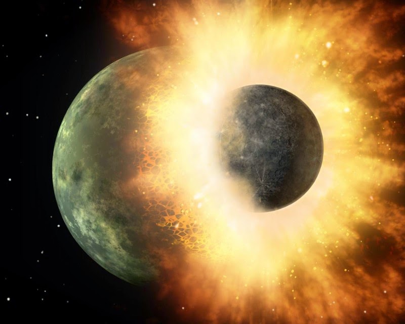
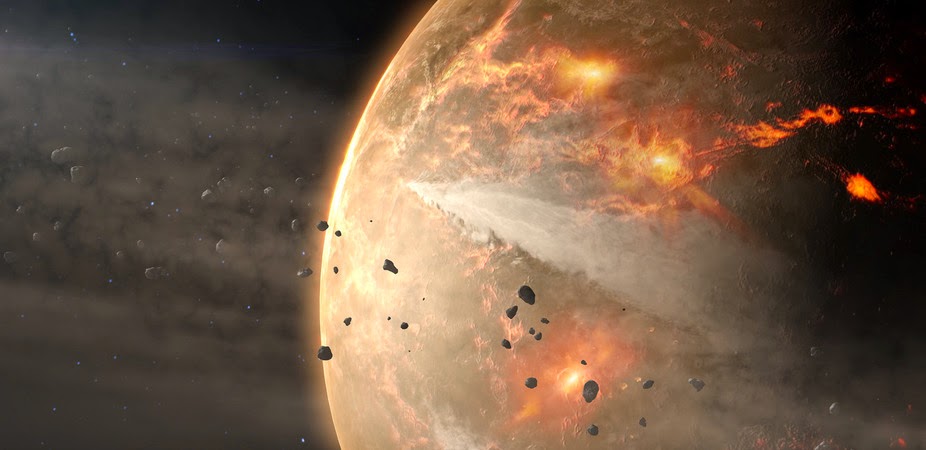
This artist’s rendering shows the collision of two planetary bodies. A collision like this is believed to have formed the moon within the first 150 million years after our solar system formed. Credit: NASA/JPL-Caltech
Within the first 150 million years after our solar system formed, a giant body roughly the size of Mars struck and merged with Earth, blasting a huge cloud of rock and debris into space. This cloud would eventually coalesce and form the moon.
For almost 30 years, planetary scientists have been quite happy with this explanation–with one major exception. Although this scenario makes sense when you look at the size of the moon and the physics of its orbit around Earth, things start to break down a little when you compare their isotopic compositions–the geological equivalent of a DNA “fingerprint.” Specifically, Earth and the moon are too much alike.
The expectation has long been that the moon should carry the isotopic “fingerprint” of the foreign body, which scientists have named Theia. Because Theia came from elsewhere in the solar system, it probably had a much different isotopic fingerprint than early Earth.
Now, a team of scientists at the University of Maryland has generated a new isotopic fingerprint of the moon that could provide the missing piece of the puzzle. By zeroing in on an isotope of Tungsten present in both the moon and Earth, the UMD team is the first to reconcile the accepted model of the moon’s formation with the unexpectedly similar isotopic fingerprints of both bodies. The results suggest that the impact of Theia into early Earth was so violent, the resulting debris cloud mixed thoroughly before settling down and forming the moon. The findings appear in the April 8, 2015 advance online edition of the journal Nature.
“The problem is that Earth and the moon are very similar with respect to their isotopic fingerprints, suggesting that they are both ultimately formed from the same material that gathered early in the solar system’s history,” said Richard Walker, a professor of geology at UMD and co-author of the study. “This is surprising, because the Mars-sized body that created the moon is expected to have been very different. So the conundrum is that Earth and the moon shouldn’t be as similar as they are.”
Several different theories have emerged over the years to explain the similar fingerprints of Earth and the moon. Perhaps the impact created a huge cloud of debris that mixed thoroughly with the Earth and then later condensed to form the moon. Or Theia could have, coincidentally, been isotopically similar to young Earth. A third possibility is that the moon formed from Earthen materials, rather than from Theia, although this would have been a very unusual type of impact.
To tease out an explanation, Walker and his team looked to another well-documented phenomenon in the early history of the solar system. Evidence suggests that both Earth and the moon gathered additional material after the main impact, and that Earth collected more of this debris and dust. This new material contained a lot of Tungsten, but relatively little of this was of a lighter isotope known as Tungsten-182. Taking these two observations together, one would expect that Earth would have less Tungsten-182 than the moon.
Sure enough, when comparing rocks from the moon and Earth, Walker and his team found that the moon has a slightly higher proportion of Tungsten-182. The key, however, is how much.
“The small, but significant, difference in the Tungsten isotopic composition between Earth and the moon perfectly corresponds to the different amounts of material gathered by Earth and the moon post-impact,” Walker said. “This means that, right after the moon formed, it had exactly the same isotopic composition as Earth’s mantle.”
This finding supports the idea that the mass of material created by the impact, which later formed the moon, must have mixed together thoroughly before the moon coalesced and cooled. This would explain both the overall similarities in isotopic fingerprints and the slight differences in Tungsten-182.
It also largely rules out the idea that the Mars-sized body was of similar composition, or that the moon formed from material contained in the pre-impact Earth. In both cases, it would be highly unlikely to see such a perfect correlation between Tungsten-182 and the amounts of material gathered by the moon and Earth post-impact.
“This result brings us one step closer to understanding the close familial relationship between Earth and the moon,” Walker said. “We still need to work out the details, but it’s clear that our early solar system was a very violent place.”
Reference:
Mathieu Touboul, Igor S. Puchtel, Richard J. Walker. Tungsten isotopic evidence for disproportional late accretion to the Earth and Moon. Nature, 2015; DOI: 10.1038/nature14355
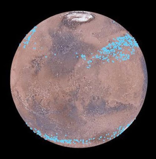
Mars distinct polar ice caps, but Mars also has belts of glaciers at its central latitudes — between the blue lines, in both the southern and northern hemispheres. A thick layer of dust covers the glaciers, so they appear as the surface of the ground, but radar measurements show that there are glaciers composed of frozen water underneath the dust. Credit: Mars Digital Image Model, NASA/Nanna Karlsson
Mars has distinct polar ice caps, but Mars also has belts of glaciers at its central latitudes in both the southern and northern hemispheres. A thick layer of dust covers the glaciers, so they appear as surface of the ground, but radar measurements show that underneath the dust there are glaciers composed of frozen water. New studies have now calculated the size of the glaciers and thus the amount of water in the glaciers. It is the equivalent of all of Mars being covered by more than one meter of ice. The results are published in the scientific journal, Geophysical Research Letters.
Several satellites orbit Mars and on satellite images, researchers have been able to observe the shape of glaciers just below the surface. For a long time scientists did not know if the ice was made of frozen water (H2O) or of carbon dioxide (CO2) or whether it was mud.
Using radar measurements from the NASA satellite, Mars Reconnaissance Orbiter, researchers have been able to determine that is water ice. But how thick was the ice and do they resemble glaciers on Earth?
A group of researchers at the Niels Bohr Institute have now calculated this using radar observations combined with ice flow modelling.
Data combined with modelling
“We have looked at radar measurements spanning ten years back in time to see how thick the ice is and how it behaves. A glacier is after all a big chunk of ice and it flows and gets a form that tells us something about how soft it is. We then compared this with how glaciers on Earth behave and from that we have been able to make models for the ice flow,” explains Nanna Bjørnholt Karlsson, a postdoc at the Centre for Ice and Climate at the Niels Bohr Institute at the University of Copenhagen.
Nanna Bjørnholt Karlsson explains that earlier studies have identified thousands of glacier-like formations on the planet. The glaciers are located in belts around Mars between the latitudes 300-500 — equivalent to just south of Denmark’s location on Earth. The glaiciers are found on both the northern and southern hemispheres.
From some locations on Mars they have good detailed high-resolution data, while they only have more sparse data from other areas. But by supplementing the sparse data with information about the flow and form of the glaciers from the very well studied areas, they have been able to calculate how thick and voluminous the ice is across the glacier belts.
Could cover the entire planet
“We have calculated that the ice in the glaciers is equivalent to over 150 billion cubic meters of ice — that much ice could cover the entire surface of Mars with 1.1 meters of ice. The ice at the mid-latitudes is therefore an important part of Mars’ water reservoir,” explains Nanna Bjørnholt Karlsson.
That the ice has not evaporated out into space could actually mean that the thick layer of dust is protecting the ice. The atmospheric pressure on Mars is so low that water ice simply evaporates and becomes water vapour. But the glaciers are well protected under the thick layer of dust.
Reference:
N. B. Karlsson, L. S. Schmidt, C. S. Hvidberg. Volume of Martian mid-latitude glaciers from radar observations and ice-flow modelling. Geophysical Research Letters, 2015; DOI: 10.1002/2015GL063219
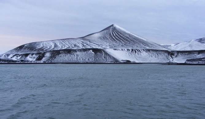
Deception wrong-footed scientists three times in ten years, and remains a mystery. Credit: Wikimedia
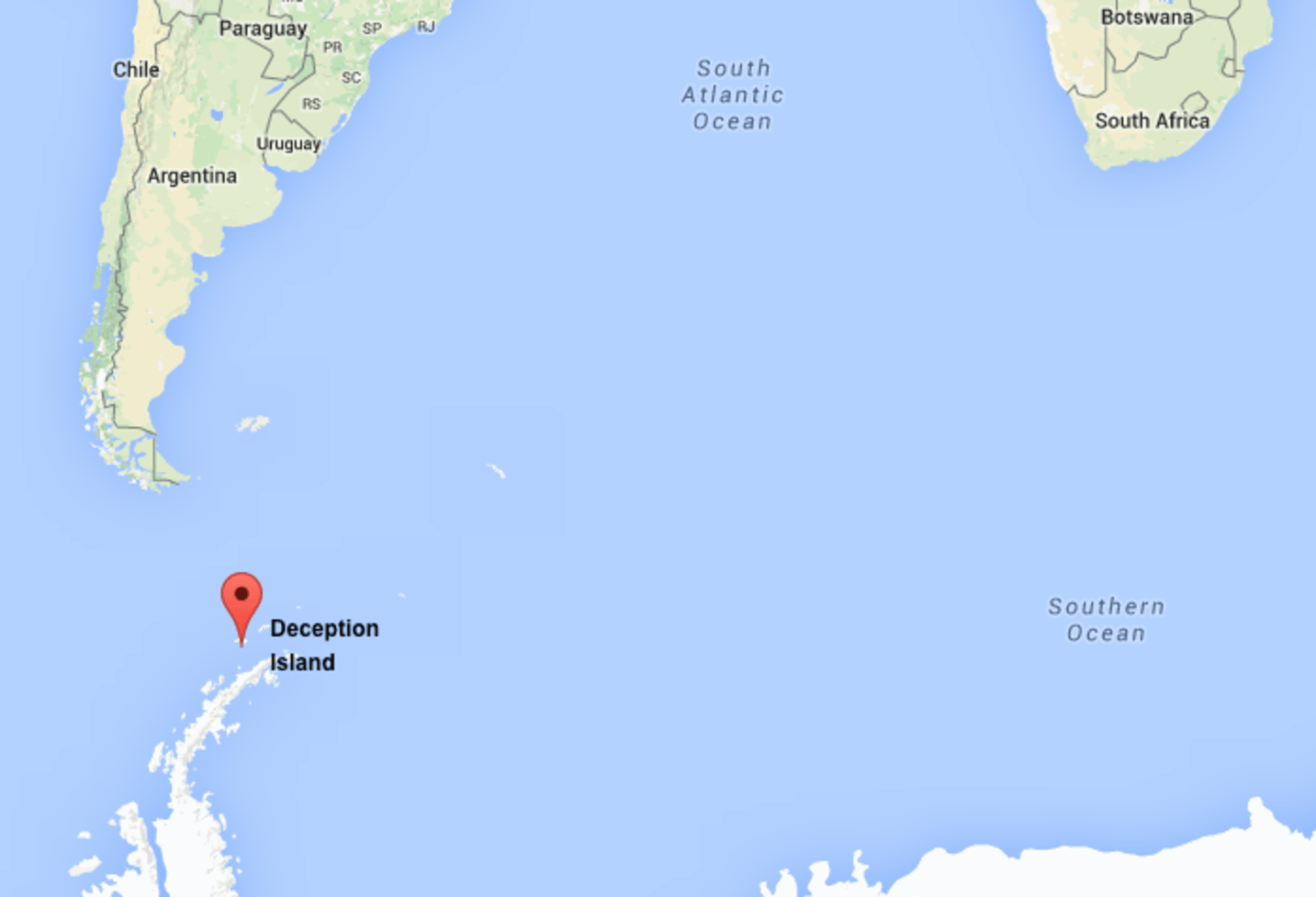
Only two volcanoes in Antarctica are active. There is Mount Erebus, which is roughly due south of New Zealand, and Deception Island, which lies about 850km south east of Cape Horn.
Mt Erebus has been erupting continuously over the last few decades. Yet the rather smaller Deception Island, in the South Shetland archipelago, is responsible for the largest known eruption in the Antarctic area.
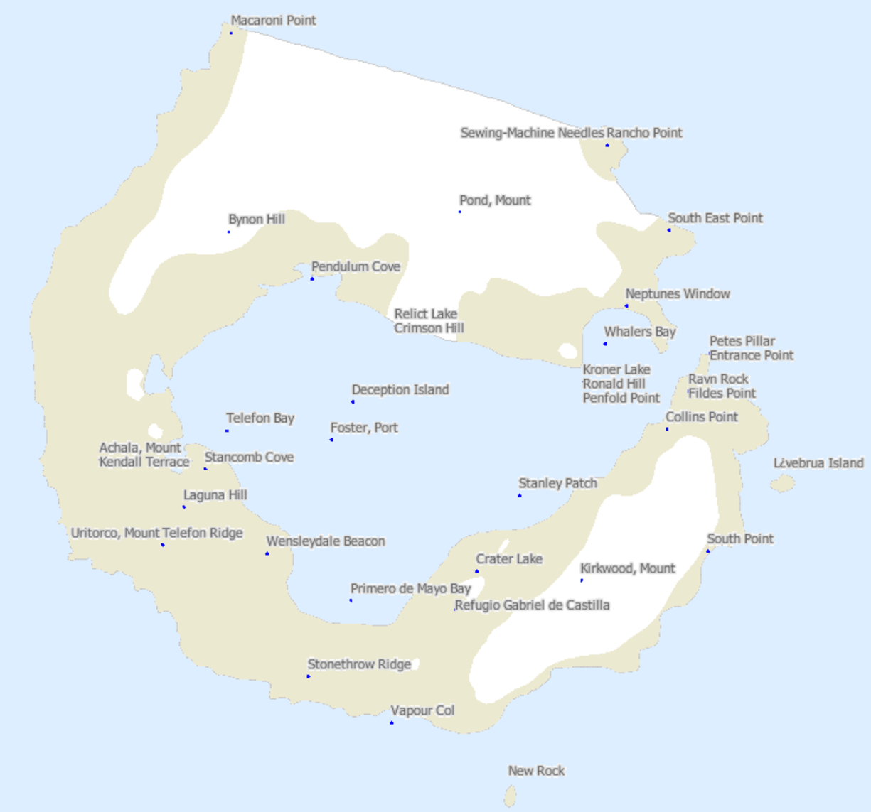
This horseshoe-shaped cauldron-like structure, or caldera, was produced more than 10,000 years ago by an explosive eruption that scattered more than 30km³ of molten rock. The result is an enclosed welcoming bay called Port Foster.
Deception was officially discovered by the British sealing captain William Smith in 1820 and was subsequently used for purposes such as seal hunting and whaling before finding its modern calling as a site for science and tourism. Maybe because you cannot see most of the volcano above the sea, tourists rarely appreciate its hidden destructive potential.
The big blunder
Claimed in the past by the UK, Chile and Argentina, it provides a unique enclosed environment in which to monitor a “volcano under the ice”. All three of those aforementioned countries financed observatories there in the 1960s (Spain added its own in 2000).
Yet two consecutive volcanic eruptions in 1967 and 1969 went unpredicted – remarkable failures in the history of volcano monitoring. Only the Argentinian and the Spanish observatories still exist.
Mud from down below
Deception Island from above. Credit: Wikimedia
The volcanic events at Deception fall into a rare category called subglacial eruptions. The island is situated in a place where there is a glacier on the ocean floor about 100m thick. Scientists would normally expect that if this were hit by lava from below, it would evaporate benignly into steam.
But the lava moving upwards at Deception has several qualities that made things happen differently: it moves slowly and it has high water content. This meant that it turned the glacier into meltwater as well as steam, creating a large overflow of mud to the surface. This was the main cause of the destruction of the UK and Chilean stations.
The reason why this melting was unexpected was because in scientific terms the glacier was “deceptively thin”. The scientists were not expecting it to produce much more than steam. Ironically, the absence of larger glaciers is what made the island the most hospitable location in Antarctica.
We understand these subglacial eruptions much better now than we did in the 1960s. Nowadays there are hazard maps to make visitors aware of the higher-risk spots on the island.
The Deception enigma
Credit: Google Maps
Yet from a volcanic point of view, Deception is a great puzzle. Many volcanoes are caused by subduction, which is where two of the Earth’s tectonic plates crash against one another, sending one plate down and pushing the other upwards. A classic example is the Cascade range in the north-western US, whose most famous volcano is Mt St Helens. The ones that scientists have observed happen on land.
Most volcanoes at sea are like Hawaii and the Azores, which we describe as hot spots. Instead of taking place near the points between tectonic plates, these are holes in the ocean floor where there is a direct line to the Earth’s mantle. The same goes for submerged calderas in the middle of the ocean, of which there are some examples near Japan.
For a time, scientists thought that Deception might be an unusual example of subduction happening in the ocean. But a more recent hypothesis is that the South Shetlands may be what we call a rift zone. This would mean that it is on a point where plates meet, but instead of colliding, there are gaps from them moving away from each other, creating new oceanic crust in the process. A good example of a rift zone is the Iceland, as can be seen in the video eruption below.
The hydrocarbon connection
Detailed geophysical surveys have been carried out across Deception since 2000, mainly financed by Spanish projects. UK geological research on the island has also been extensive.
You may be wondering why governments have spent so much on research there. Don’t be fooled into thinking that this is some kind of place of virtue where different nations fund research just to understand how our Earth works.
Rifts fill up with the remains of volcanic explosions and other sediment eroded from the margins of the valley. This process is critical for the production of oil. Located at the western edge of the arc, Deception is the ideal place to observe rift processes because of the natural harbour, which shelters scientists from the harsh Antarctic weather.
Rifting is the reason for all the oil in the North Sea. The oil is not deposited where the rift is located, but some distance away. In the same way, there is almost no likelihood of an oil discovery on Deception. But understanding the process of rifting there will be a strong indication that there is oil to the north of the South Shetland Islands. It would also confer an exploration advantage worldwide – so Deception without oil is as valuable as Deception with oil.
So Deception could be the key to unveiling how rifts form and where oil is, in places where resources are unexploited. In an era where the political claims to the Antarctic have long since receded, that should ensure that this frozen corner of the world remains important for some time to come.
Video
Note : The above story is based on materials provided by The Conversation. This story is published courtesy of The Conversation (under Creative Commons-Attribution/No derivatives).
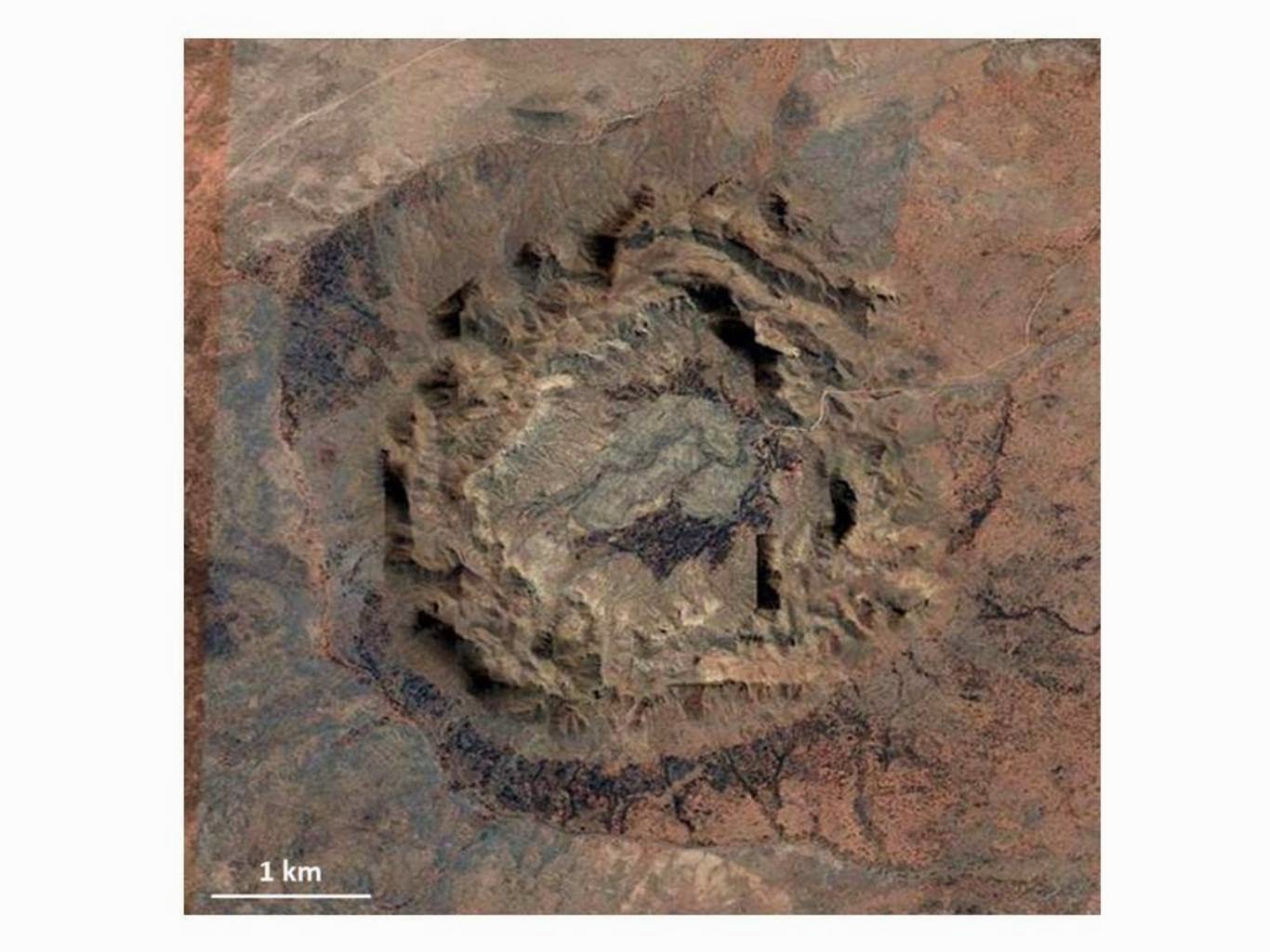
Our solar system is far from empty. A rogue asteroid or comet may have been responsible for the largest impact site yet discovered in Warburton in central Australia. Credit: NASA Goddard Space Flight Center, CC BY-SA
Not long ago, asteroid impacts weren’t considered as a significant factor in the evolution of Earth. Following the Late Heavy Bombardment, which pummelled the inner solar system around 3.8 billion to 3.9 billion years ago, asteroid impacts were generally regarded as minor events.
All this changed in the late 1970s, when Walter and Louis Alvarez discovered the 65-million-year-old K-T (Cretaceous-Tertiary boundary) asteroid impact event. This is now known to be linked to the extinction of the dinosaurs, among many other species.
Thus interest in extra-terrestrial impact research – a discipline bridging astronomy and geology – soared when the spectre of dinosaurs escaping asteroid impact-ignited flames was transformed from science fiction to science fact.
Attention has now been drawn to our own shores with the discovery of new impact structures, including two very large asteroid impacts buried more than two kilometres under the surface in northeastern South Australia.
If the preliminary evidence is anything to go by, these could represent the largest impact sites on the planet. One can only imagine the catastrophic event that might have caused them, and the consequences it had for life on Earth at the time.
Heavy rain
The impressive Gosses Bluff impact structure in the Northern Territory, which is dates at 142 million years-old. Author provide
To date researchers have identified more than 172 meteorite craters and asteroid impact structures around the world, showing that our planet has never been spared from bombardment by asteroids. Most of the asteroids responsible for these impacts have originated from the asteroid belt between Mars and Jupiter and most of the comets originated from the Oort cloud at the fringe of the solar system.
Here in Australia, we are blessed with a truly ancient landscape, some of which is up to 3.7 billion years old and contains minerals up to 4.4 billion years old. We also have as high degree of geological stability, meaning many of the impact structures have been preserved over the ages.
To date, a total of 33 impact craters and 27 probable-to-likely impact structures have been found in Australia, ranging from small crater clusters such as Henbury, Northern Territory, to large impact structures such as Acraman in South Australia and Woodleigh in Western Australia.
Some of these are well exposed, such as Gosses Bluff, Northern Territory, Spider in the Kimberley and Lawn Hill in Queensland. Others are buried by younger sediments, such as Woodleigh, Western Australia, Yallalie in Western Australia and Tookoonooka and Talundilly in southwest Queensland.
But the largest of them all may have been uncovered under the red expanse of central Australia.
Double impact
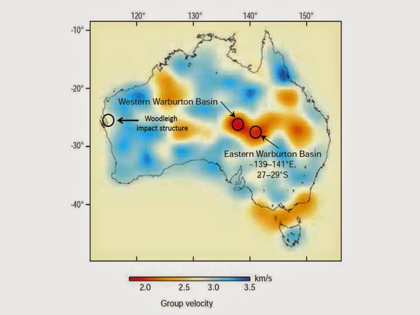
Those red splodges show seismic anomalies which coincide with the Warburton structures in north eastern South Australia. These anomalies represent large scars in the Earth crust. Author provided
The first hint at shock metamorphism of the Earth crust in north eastern South Australia was discovered when Tonguc Uysal at the University of Queensland’s Geothermal Energy Centre of Excellence was involved in drilling for geothermal energy in 2009 in the oil and gas rich Cooper Basin, which overlies the Warburton Basin.
While there, he came across telltale evidence of unusual micro-structures within quartz grains from the local granites. He recognised the quartz structures were similar to those that I and my colleagues found in 1999 in the 120 kilometre large impact structure at Woodleigh in Western Australia.
I was intrigued by Tonguc’s findings, and he subsequently offered me the opportunity to analyse the drill core samples myself.
Starting in 2010 I spent many months studying drill core samples from the Warburton Basin, using three-dimensional optical microscopy and scanning electron microscopy. This was followed by detailed transmission electron microscopy undertaken by John Fitzgerald.
We found that the quartz lamella displayed the characteristic deformation pattern which can only be produced by extreme shock pressures above 10 gigapascals (100 kilobars). To put this in perspective, these levels are much greater than the pressures at the base of the continental crust 30km to 50km beneath the Earth’s surface.
Analysis of the Warburton samples suggested shock pressures of between 10 and 20 gigapascals, which can only be produced by an impact by a large asteroid or a comet.
While we were performing our analyses, seismic researchers Brian Kennett and Erdinc Saygin and their colleagues at the Australian National University published a paper reporting very large seismic anomalies in north-eastern South Australia. These anomalies coincide with the region where we found shock features in quartz crystals.
The seismic evidence may be related to deep fracturing of the crust and to an increased geothermal gradient, where the temperature increases more rapidly with depth than in other regions of the Australian continent. This observation was consistent with geophysical modelling of airborne magnetic and gravity data which indicate anomalies under the Cooper Basin, studied by Tony Meixner of Geoscience Australia.
Piecing the evidence together
Using the geophysical anomalies along with the distribution of shocked quartz grains found in drill holes, we estimate the combined size of the twin structures at approximately 400 km. This would make the Warburton twin structures the largest known to date.
However, we are yet to pinpoint the age and the consequences of the Warburton twin impacts. What we do know is the impact must be at least 300 million years old or older. This is based on study of the ages of bodies of granite affected by the impact, which are overlain by younger sediments that show no signs of shock.
Other studies of the cores of zircons in the granite by Tonguc Uysal and Alexander Middleton and their students at the University of Queensland suggest the zircons contain signatures of both a 300 million years old impact and a 420 million years old impact.
If we can resolve the age question, that will allow us to search for fallout ejected from the original crater and related tsunami events, and potentially figure out whether the impacts are related to an extinction event.
The geological record contains a number of extinction events that were associated with impacts by asteroids, such as the 580 million years old Acraman impact event and the 66 million years old Cretaceous–Paleogene event that killed off the dinosaurs.
The most significant mass extinction event, though, is the massive Permian-Triassic extinction which killed off 90% of species alive around 250 million years ago. This was a period of intense volcanic activity and also coincides with the Araguainha impact located in Brazil.
The discovery of the Warburton twin impacts constitutes a milestone in the study of the impact history of Earth, including research of impact events associated with 2.5 billion to 3.5 billion years old formations in the Pilbara Craton in Western Australia. The more we know about these impacts, the better we can understand other phenomena, such as mass extinctions, the formation of certain geological structures over time and related magmatic events.
It also paints a vivid picture of what might have happened on that fateful day a few hundred million years ago, and the catastrophe it must have wrought.
Note : The above story is based on materials provided by The Conversation. This story is published courtesy of The Conversation (under Creative Commons-Attribution/No derivatives).
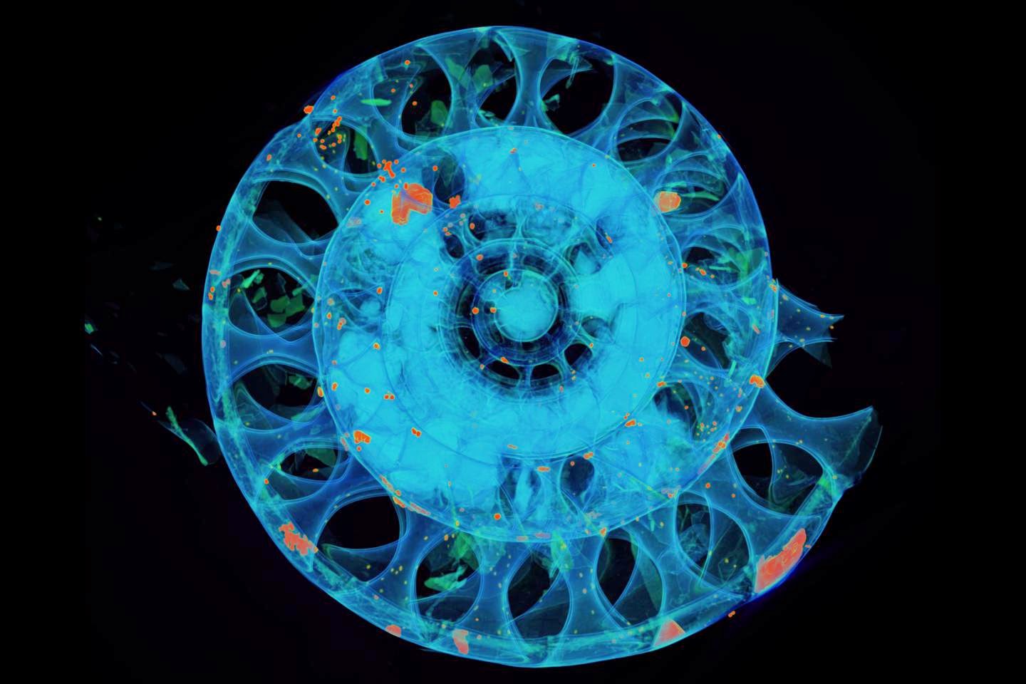
Using high-resolution x-ray radiation, Bochum-based researchers study extinct marine creatures. Depicted here is a fossil ammonite. Credit: RUBIN, image: René Hoffmann
Using state-of-the-art imaging techniques, palaeontologists at the Ruhr-Universität Bochum (RUB) have been examining extinct marine creatures. Quantitative analyses provide new evidence that ammonites were able to swim using their shell – very much like the recent nautilus. For the purpose of the study, the researchers, together with partners from the industry, developed an evaluation process for high-res CT images. The science magazine “RUBIN” reports about the results.
Method established using the shell of recent nautilus
Ammonites had a visceral mass that was protected by a helical shell with several chambers. One theory postulates that the creatures lived at the bottom of the sea. Another claims that they were able to swim by using their shell with its gas-filled chambers to compensate for the weight of their shell and soft body, rendering them neutrally buoyant. Together with his team, RUB researcher Dr René Hoffmann investigated how much buoyancy an ammonite shell could generate. First, the palaeontologists from Bochum developed a reliable evaluation technique for their CT images, using the nautilus shells as a test object. Their method now enables them to precisely ascertain the volumes of the examined shells and to calculate their weight, as well as the volumes of the gas-filled chambers. The data thus gathered indicate the buoyancy generated by the shell. In order to clarify if the ammonites were able to swim, the researchers need to know if their shell provides sufficient buoyancy to compensate the weight of the visceral mass and the shell. They estimated the latter, basing it on observations of the nautilus animal.
Technique requires special fossils
For the CT analysis, René Hoffmann needed hollow fossilised ammonites. In order to find them, he travelled to Russia and Japan, to name but two. Together with PhD student Robert Lemanis, he analysed a 0.98 millimetres large ammonite hatchling. The result: three to five gas-filled shell chambers would have been sufficient to enable the ammonites to swim freely in the water directly after hatching. The examined shell had eleven chambers. How many of them existed in the moment of hatching, however, cannot be ascertained – the larger the molluscs became, the more chambers they created. Still, the RUB analyses showed that the hatchling would not have been condemned to dwelling at the bottom, even if only one chamber had been filled with gas; using active swimming motions, the young ammonite would have been able to move around freely in water and stop itself from sinking.
Reference:
R. Lemanis, S. Zachow, F. Fusseis, R. Hoffmann (2015): A new approach using high-resolution computed tomography to test the buoyant properties of chambered cephalopod shells, Paleobiology, DOI: 10.1017/pab.2014.17
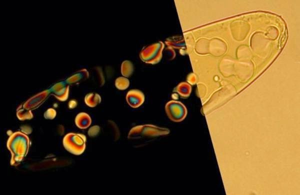
The image shows a droplet of condensed nano-DNA and within it smaller drops of its liquid crystal phase which show up in polarized light on the left. The liquid crystal droplets act as ‘micro-reactors’. Credit: Noel Clark, University of Colorado
The self-organization properties of DNA-like molecular fragments four billion years ago may have guided their own growth into repeating chemical chains long enough to act as a basis for primitive life, says a new study by the University of Colorado Boulder and the University of University of Milan.
While studies of ancient mineral formations contain evidence for the evolution of bacteria from 3.5 to 3.8 billion years ago — just half a billion years after the stabilization of Earth’s crust — what might have preceded the formation of such unicellular organisms is still a mystery. The new findings suggest a novel scenario for the non-biological origins of nucleic acids, which are the building blocks of living organisms, said CU-Boulder physics Professor Noel Clark, a study co-author.
A paper on the subject led by Tommaso Bellini of the University of Milan was published in a recent issue of Nature Communications. Other CU-Boulder co-authors of the study include Professor David Walba, Research Associate Yougwooo Yi and Research Assistant Gregory P. Smith. The study was funded by the Grant PRIN Program of the Italian Ministries of Education, Universities and Research and by the U.S. National Science Foundation.
The discovery in the 1980’s of the ability of RNA to chemically alter its own structure by CU-Boulder Nobel laureate and Distinguished Professor Tom Cech and his research team led to the development of the concept of an “RNA world” in which primordial life was a pool of RNA chains capable of synthesizing other chains from simpler molecules available in the environment. While there now is consensus among origin-of-life researchers that RNA chains are too specialized to have been created as a product of random chemical reactions, the new findings suggest a viable alternative, said Clark.
The new research demonstrates that the spontaneous self-assembly of DNA fragments just a few nanometers in length into ordered liquid crystal phases has the ability to drive the formation of chemical bonds that connect together short DNA chains to form long ones, without the aid of biological mechanisms. Liquid crystals are a form of matter that has properties between those of conventional liquids and those of a solid crystal — a liquid crystal may flow like a liquid, for example, but its molecules may be oriented more like a crystal.
“Our observations are suggestive of what may have happened on the early Earth when the first DNA-like molecular fragments appeared,” said Clark.
For several years the research group has been exploring the hypothesis that the way in which DNA emerged in the early Earth lies in its structural properties and its ability to self-organize. In the pre-RNA world, the spontaneous self-assembly of fragments of nucleic acids (DNA and RNA) may have acted as a template for their chemical joining into polymers, which are substances composed of a large number of repeating units.
“The new findings show that in the presence of appropriate chemical conditions, the spontaneous self assembly of small DNA fragments into stacks of short duplexes greatly favors their binding into longer polymers, thereby providing a pre-RNA route to the RNA world,” said Clark.
Reference:
Tommaso P. Fraccia, Gregory P. Smith, Giuliano Zanchetta, Elvezia Paraboschi, Yougwooo Yi, David M. Walba, Giorgio Dieci, Noel A. Clark, Tommaso Bellini. Abiotic ligation of DNA oligomers templated by their liquid crystal ordering. Nature Communications, 2015; 6: 6424 DOI: 10.1038/ncomms7424
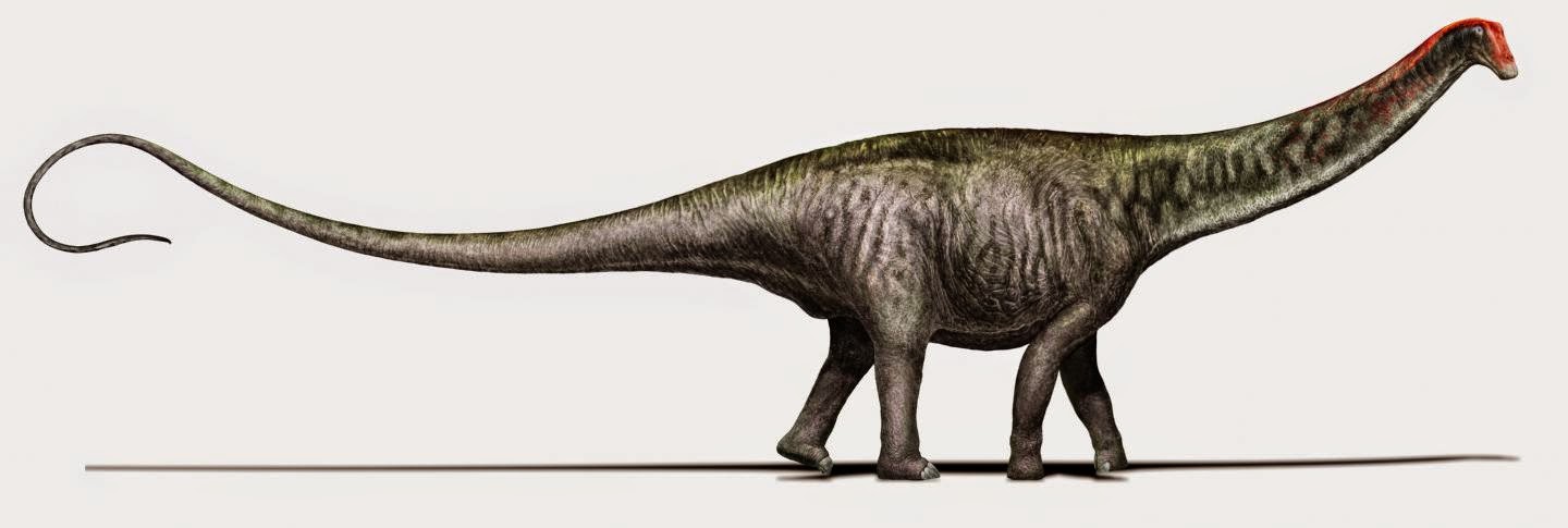
This is Brontosaurus as researchers see it today — with a Diplodocus-like head. Credit: Davide Bonadonna, Milan, Italy
Although well known as one of the most iconic dinosaurs, Brontosaurus (the ‘thunder lizard’) has long been considered misclassified. Since 1903, the scientific community has believed that the genus Brontosaurus was in fact the Apatosaurus. Now, an exhaustive new study by palaeontologists from Portugal and the UK provides conclusive evidence that Brontosaurus is distinct from Apatosaurus and as such can now be reinstated as its own unique genus.
Brontosaurus is one of the most charismatic dinosaurs of all time, inspiring generations of children thanks to its size and evocative name. However, as every armchair palaeontologist knows, Brontosaurus was in fact a misnomer, and it should be correctly referred to as Apatosaurus. At least, this is what scientists have believed since 1903, when it was decided that the differences between Brontosaurus excelsus and Apatosaurus were so minor that it was better to put them both in the same genus. Because Apatosaurus was named first, it was the one that was used under the rules of scientific naming.
In fact, of course, the Brontosaurus was never really gone – it was simply treated as a species of the genus Apatosaurus: Apatosaurus excelsus. So, while scientists thought the genus Brontosaurus was the same as Apatosaurus, they always agreed that the species excelsus was different from other Apatosaurus species. Now, palaeontologists Emanuel Tschopp, Octávio Mateus, and Roger Benson say that Brontosaurus was a unique genus all along. But let’s start from the beginning.
The history of Brontosaurus is complex, and one of the most intriguing stories in science. In the 1870s, the Western United States formed the location for dozens of new finds of fossil species, most notably of dinosaurs. Field crews excavated numerous new skeletons mostly for the famous and influential palaeontologists Marsh and Cope. During that period, Marsh’s team discovered two enormous, partial skeletons of long-necked dinosaurs and shipped them to the Yale Peabody Museum in New Haven, where Marsh worked. Marsh described the first of these skeletons as Apatosaurus ajax, the “deceptive lizard” after the Greek hero Ajax. Two years later, he named the second skeleton Brontosaurus excelsus, the “noble thunder lizard”. However, because neither of the skeletons were found with a skull, Marsh reconstructed one for Brontosaurus excelsus. Brontosaurus was a massive animal, like Apatosaurus, and like another long-necked dinosaur from the Western United States, Camarasaurus. Because of this similarity, it seemed logical at the time that Brontosaurus had a similarly stout, box-like skull to that of Camarasaurus. However, this reconstruction was later found to be wrong.
Shortly after Marsh’s death, a team from the Field Museum of Chicago found another skeleton similar to both Apatosaurus ajax and Brontosaurus excelsus. In fact, this skeleton was intermediate in shape in many aspects. Therefore, palaeontologists thought that Brontosaurus excelsus was actually so similar to Apatosaurus ajax that it would be more correct to treat them as two different species of the same genus. It was the second extinction of Brontosaurus – a scientific one: from now on, Brontosaurus excelsus became known as Apatosaurus excelsus and the name Brontosaurus was not considered scientifically valid any more.
The final blow to “Brontosaurus” happened in the 1970s, when researchers showed that Apatosaurus was not closely related to Camarasaurus, but to yet another dinosaur from the same area: Diplodocus. Because Diplodocus had a slender, horse-like skull, Apatosaurus and thus also “Brontosaurus” must have had a skull more similar to Diplodocus instead of to Camarasaurus – and so the popular, but untrue myth about “Brontosaurus” being an Apatosaurus with the wrong head was born.
But now, in a new study published in the peer reviewed open access journal PeerJ and consisting of almost 300 pages of evidence, a team of scientists from Portugal and the UK have shown that Brontosaurus was distinct from Apatosaurus after all – the thunder lizard is back!
How can a single study overthrow more than a century of research? “Our research would not have been possible at this level of detail 15 or more years ago”, explains Emanuel Tschopp, a Swiss national who led the study during his PhD at Universidade Nova de Lisboa in Portugal, “in fact, until very recently, the claim that Brontosaurus was the same as Apatosaurus was completely reasonable, based on the knowledge we had.” It is only with numerous new findings of dinosaurs similar to Apatosaurus and Brontosaurus in recent years that it has become possible to undertake a detailed reinvestigation of how different they actually were.
In science, the distinction between species and genera is without clear rules. Does this mean that the decision to resurrect Brontosaurus is just a matter of personal preference? “Not at all”, explains Tschopp, “we tried to be as objective as possible whenever making a decision which would differentiate between species and genus”. The researchers applied statistical approaches to calculate the differences between other species and genera of diplodocid dinosaurs, and were surprised by the result. “The differences we found between Brontosaurus and Apatosaurus were at least as numerous as the ones between other closely related genera, and much more than what you normally find between species,” explained Roger Benson, a co-author from the University of Oxford.
Therefore, Tschopp and colleagues have concluded that it is now possible to resurrect Brontosaurus as a genus distinct from Apatosaurus. “It’s the classic example of how science works”, said Professor Mateus, a collaborator on the research. “Especially when hypotheses are based on fragmentary fossils, it is possible for new finds to overthrow years of research.”
Science is a process, always moving towards a clearer picture of the world around us. Sometimes this also means that we have to step backwards a bit before we continue to advance. That’s what keeps the curiosity going. Hence, it is fitting that the Brontosaurus which sparked the curiosity of millions of people worldwide has now returned to do so again.
Reference:
A specimen-level phylogenetic analysis and taxonomic revision of Diplodocidae (Dinosauria, Sauropoda). Emanuel Tschopp, Octávio Mateus, Roger B.J. Benson. DOI: 10.7717/peerj.857
Note : The above story is based on materials provided by PeerJ.
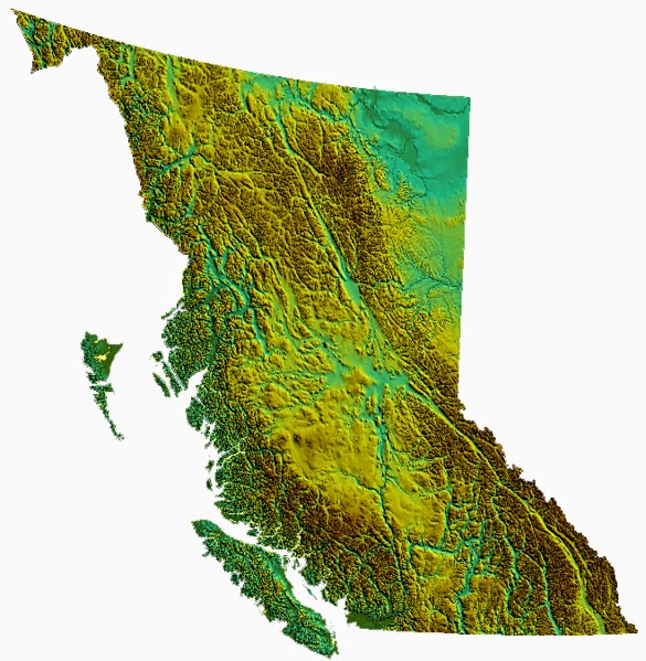
The Pacific and North America plate boundary off the coast of British Columbia and southeastern Alaska is a complex system of faults capable of producing very large earthquakes. The recent 2012 Mw 7.8 Haida Gwaii and 2013 Mw 7.5 Craig earthquakes released strain built up over years, but did not release strain along the Queen Charlotte Fault, which remains the likely source of a future large earthquake, according to reports published in a special issue of the Bulletin of the Seismological Society of America (BSSA).
“The study of these two quakes revealed rich details about the interaction between the Pacific and North America Plates, advancing our understanding of the seismic hazard for the region,” said Thomas James, research scientist at Geological Survey of Canada and one of the guest editors of the special issue, which includes 19 technical articles on both the Haida Gwaii and Craig events.
The Haida Gwaii and Craig earthquakes offered new information about the tectonic complexity of the region. Prior to the 2012 earthquake, the Queen Charlotte Fault, a strike-slip fault similar to the San Andreas Fault in California, was the dominating tectonic structure in the area.
Nykolaishen et al. used GPS observations of crustal motion to locate the earthquake’s rupture offshore to the west of Haida Gwaii, rather than beneath the islands. A close study of the Haida Gwaii mainshock by Kao et al. revealed the Pacific plate slid at a low angle below the North American plate on a previously suspected thrust fault, confirming the presence of subduction activity in the area.
“This was an event the thrust interface of the plate boundary system, confirming that there is a subduction system in the Haida Gwaii area,” said Honn Kao, seismologist with the Geological Survey of Canada, who, along with his colleagues, examined the source parameters–causative faults, rupture processes and depths–of the mainshock and sequence of strong aftershocks.
“The implication of a confirmed subduction zone is that in addition to the Queen Charlotte Fault, we now have another source which can produce devastating megathrust earthquakes in the area,” said Kao.
The aftershocks clustered around the periphery of the rupture zone, both on the seaward and landward side of the plate boundary and reflected normal faulting behavior–caused by the bending, extending or stretching of rock– rather than the thrust faulting of the mainshock.
“Our observations of normal faulting imply that the mainshock of the Haida Gwaii earthquake dramatically altered the stress field in the rupture zone, especially in a neighboring region,” said Kao.
The distribution of aftershocks occurred to the north of a previously identified seismic gap where large earthquakes have not occurred in historic times. The gap is located to the south of the where 1949 M8.1 Queen Charlotte earthquake ruptured. Though the Haida Gwaii earthquake may have activated some part of the Queen Charlotte Fault, said Kao, it was limited and did not relieve stress along the seismic gap.
The Haida Gwaii rupture shook southeastern Alaska, and the northwest directivity of ground motion may have influenced the timing of the January 2013 Craig earthquake, suggests James et al. in the introduction to the overall special issue.
A report by Stephen Holtkamp and Natalia Ruppert at the University of Alaska Fairbanks examines 1785 aftershocks in the Craig earthquake sequence, identifying a mix of faulting behavior that suggests the region is still in a state of transpression–the plates are both sliding past each other and colliding at an angle.
The articles in this special issue will appear in print in early May and online in April. The special issue features three main themes. The regional tectonic framework and the nature of the interaction between the Pacific and North America plates at the Queen Charlotte Fault zone are presented in five papers. Three papers focus on the Craig earthquake and examine the main shock, aftershocks and crustal motions. Ten papers discuss the Haida Gwaii event.
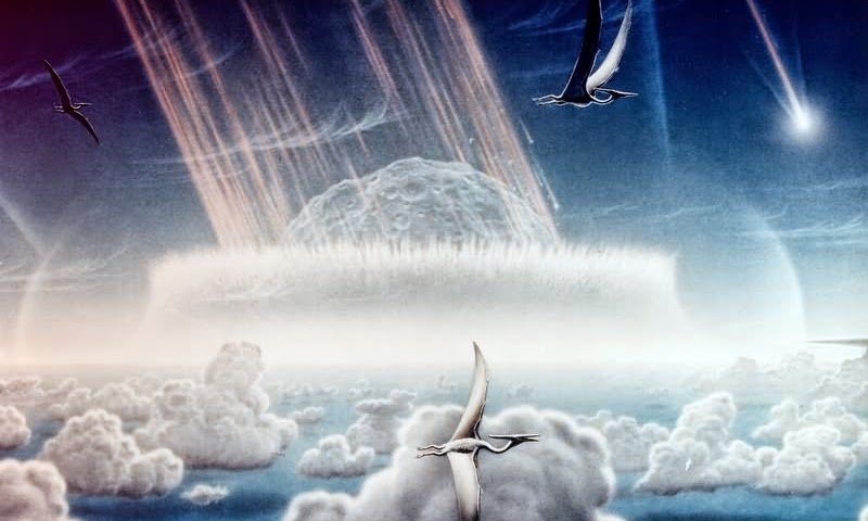
Artist’s impression of the Chicxulub asteroid impacting the Yucatan Peninsula as pterodactyls fly in the sky above. Painting by Donald E. Davis. Credit: NASA
An international research team is formalizing plans to drill nearly 5,000 feet below the seabed to take core samples from the crater of the asteroid that wiped out the dinosaurs.
The group met last week in Merida, Mexico, a city within the nearly 125-mile-wide impact site, to explain the research plans and put out a call for scientists to join the expedition planned for spring 2016. The roughly $10 million in funding for the expedition has been approved and scheduled by the European Consortium for Ocean Research Drilling (ECORD)—part of the International Ocean Discovery Program (IODP)—and the International Continental Scientific Drilling Program (ICDP).
Dinosaurs and other reptiles ruled the planet for 135 million years. That all changed 65.5 million years ago when a 9-mile-wide asteroid slammed into the Earth, triggering a series of apocalyptic events that killed most large animals and plants, and wiped out the dinosaurs and large marine reptiles. The event set the stage for mammals—and eventually humans—to take over. Yet, we have few geologic samples of the now buried impact crater.
Sean Gulick, a researcher at The University of Texas at Austin Institute for Geophysics (UTIG), and a team of scientists from the U.K. and Mexico are working to change that. The team is planning to take the first offshore core samples from near the center of the impact crater, which is called Chicxulub after the seaside village on the Yucatán Peninsula near the crater’s center.
The team, led by Gulick and Joanna Morgan of Imperial College London, will be sampling the crater’s “peak ring”—an enigmatic ring of topographically elevated rocks that surrounds the crater’s center, rises above its floor and has been buried during the past 65.5 million years by sediments.
A peak ring is a feature that is present in all craters caused by large impacts on rocky planetoids. By sampling the Chicxulub peak ring and analyzing its key features, researchers hope to uncover the impact details that set in motion one of the planet’s most profound extinctions, while also shedding light on the mechanisms of large impacts on Earth and on other rocky planets.
“What are the peaks made of? And what can they tell us about the fundamental processes of impacts, which is this dominant planetary resurfacing phenomena?” said Gulick, who is also a research associate professor at the UT Jackson School of Geosciences. UTIG is a research unit of the Jackson School.
The researchers are also interested in examining traces of life that may have lived inside the peak ring’s rocks. Density readings of the rocks indicate that they probably are heavily broken and porous—features that may have served as protected microenvironments for exotic life that could have thrived in the hot, chemically enriched environment of the crater site after impact. Additionally, the earliest recovery of marine life should be recorded within the sediments that filled in the crater in the millions of years after the impact.
“The sediments that filled in the [crater] should have the record for organisms living on the sea floor and in the water that were there for the first recovery after the mass extinction event,” Gulick said. “The hope is we can watch life come back.”
The expedition will last for two months and involve penetrating nearly 5,000 feet beneath the seabed from an offshore platform. The core will be the first complete sample of the rock layers from near the crater’s center.
Once extracted, the core will be shipped to Germany and split in two. Half will be immediately analyzed by an international team of scientists from the U.S., U.K., Mexico and other nations, and half will be saved at a core repository at Texas A&M University for future research needs by the international community.
The team also includes researchers from the National Autonomous University of Mexico (UNAM) and Centro de Investigación Científica de Yucatán (CICY). Scientists interested in joining the mission must apply by May 8, 2015. For more information on the mission and the application process, see the European Consortium for Ocean Research Drilling’s call for applications.
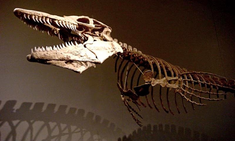
New research sheds light on the evolutionary relationships of living and extinct reptiles. This skeleton belonged to a mosasaur, a carnivorous marine lizard that died out with the dinosaurs 65 million years ago. Credit: Wikimedia Commons
A new study has helped settle the controversial relationships among the major groups of lizards and snakes, and it sheds light on the origins of a group of giant fossil lizards.
Squamate reptiles—lizards and snakes—are among the most diverse groups of vertebrates, with more than 9,000 living species. They are important for humans because venomous snakes cause tens of thousands of deaths every year. At the same time, their toxins are a critical resource for many medicines, including those for heart disease and diabetes. Lizards and snakes also are important model systems for biological research, especially in ecology and evolutionary biology.
Unfortunately, studies of squamate biology have been hampered by controversy over their evolutionary relationships, and some researchers consider their family tree to be unresolved. The problem is that studies based on traditional, anatomical characters and those based on molecular data from DNA sequences have strongly disagreed, especially on how the iguanas and their relatives (called iguanians) are related to snakes and to other groups of lizards. Iguanians include horned lizards, flying dragons and basilisks.
A new study by scientists from the University of Arizona, San Diego State University, the Smithsonian Institution, Brigham Young University and the University of Mississippi has now helped to resolve this controversy, and it also offers new insights on the evolution of fossil lizards. The results are published online in the journal PLoS One.
“Anatomical data put iguanians at the base of the tree, whereas molecular data suggest that the iguanians evolved more recently and are closely related to snakes and a group including the monitor and alligator lizards, called the anguimorphs,” said John J. Wiens, a professor in the Department of Ecology and Evolutionary Biology in the UA College of Science. “The results of our study overwhelmingly support the molecular hypothesis.”
The team assembled the largest-yet datasets of both anatomical and molecular characters for the major groups of lizards and snakes. The researchers showed that when the anatomical and molecular data are combined, the results conclusively support the molecular hypothesis, placing iguanas and relatives with snakes and anguimorphs.
One possible explanation for these results is the greater number of molecular characters relative to morphological characters (35,673 molecular versus 691 morphological). This larger number might favor the molecular hypothesis, regardless of which hypothesis is actually true. To test this idea, the researchers trimmed the molecular dataset to only 63 characters. When they analyzed this reduced molecular dataset with all 691 anatomical characters, the results still supported the molecular hypothesis, placing iguanians with snakes and anguimorphs instead of at the base of the tree.
Wiens’ team also found that there was support for the molecular hypothesis hidden in the morphological dataset. When the researchers combined the molecular and morphological data, they found that the number of morphological characters that supported the branch uniting iguanians, snakes and anguimorphs (the molecular hypothesis) was almost equal to the number placing iguanians near the base of the tree (the morphological hypothesis).
In addition, the researchers found that when they divided up the anatomical characters and analyzed each set separately, only one of the six sets clearly supported the morphological hypothesis.
“In fact, the morphological data are really ambiguous,” Wiens said. “Or in some cases, even worse than ambiguous.”
He explained that the morphological data give very strange, non-traditional relationships in which all burrowing species are placed together, including those classified in different families.
“Basically, burrowing lizards tend to evolve elongate bodies, reduced limbs and a whole suite of other anatomical traits, even if they are only distantly related to each other,” Wiens said. “Placing all burrowing species together disagrees strongly with the molecular data, and also with traditional taxonomy. In summary, the anatomical data can be widely misleading in squamate reptiles.”
Wiens and co-authors suggest a similar explanation for why the anatomical data are misleading about the placement of iguanians in particular.
According to Wiens, iguanian lizards typically capture prey using their tongue, whereas snakes and other lizards use their jaws. Scientists have documented many differences in diet, behavior and anatomy that seem to be associated with capturing prey with the tongue versus the jaw. It turns out that the closest living relative to lizards and snakes, the tuatara of New Zealand, also uses its tongue to capture prey. Therefore, the anatomical characters that place iguanians at the base of the tree may reflect parallel evolution associated with these different feedings modes.
The study also has implications for understanding the evolution of fossil lizards, such as mosasaurs, as well. These carnivorous marine lizards, which died out with the dinosaurs around 65 million years ago, have traditionally been thought to either be close relatives of monitor lizards, or close to the base of the squamate family tree. The new study combined data from both living and fossil species and revealed mosasaurs to be close relatives of snakes, and only distantly related to monitor lizards and species at the base of the tree.
“What is really interesting about this is that we have no molecular data for mosasaurs at all,” Wiens said. “Our results show how combining molecular and anatomical data can reveal evolutionary relationships of fossil species that one might not predict from the anatomical data alone.”
Reference:
“Integrated Analyses Resolve Conflicts over Squamate Reptile Phylogeny and Reveal Unexpected Placements for Fossil Taxa.” PLoS ONE 10(3): e0118199. DOI: 10.1371/journal.pone.0118199
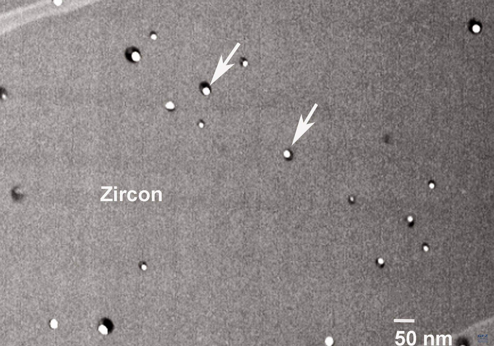
Zircon from East Antarctica with nanospheres of metallic lead under GFZ’s transmissionelectron-microscope TEM. The rock sample is more than 3,4 billion years old. Photo Credit: GFZ
Rocks do not loose their memory during Earth history but their true ages might be distorted: even under ultra high-temperature metamorphic conditions exceeding 1200°C zircon maintains its lead content accumulated during radioactive decay of uranium and thorium.
Giga year old zircon crystals still contain lead in form of nanometre size spheres of pure lead. However, the inhomogeneous spatial distribution of the lead spheres might falsify ages determined from high-resolution Pb isotope measurement with ion probe.
Zircon is an ideal mineral for age determination of very old rocks because it is believed to be a closed system during Earth history. Zircon geochronology thus is a standard method of geological age determination. Recently, an international group of earth scientists studied zircon from 3,4 billion years old high-temperature metamorphic rocks from Antarctica with transmission electron microscopy TEM at the GFZ German Research Centre for Geosciences. TEM investigations revealed that the lead from radioactive decay was not homogeneously distributed in zircon but was accumulated withinin inhomogeneously distributed Pb nano-spheres in zircon with only 5 to 30 nm in diameter. The inhomogeneous distribution of lead in zircon might adulterate the ages measured with high-spatial resolution ion probe technique.
Reference:
Monika A. Kusiak et al.: “Metallic lead nanospheres discovered in ancient zircons”, Proceedings of the National Academy of Sciences, PNAS Early Edition, 06.04.2015, DOI: doi/10.1073/pnas.1415264112
Landslides occur in all 50 states and U.S. territories, and cause $1-2 billion in damages and more than 25 fatalities on average each year. USGS scientists aim to improve our understanding of landslide hazards to help protect communities and reduce associated losses.
Video Sections:
Types of Landslides
USGS Science
Did You See It?
Debris Flow Early Warning System (NOAA Partnership)
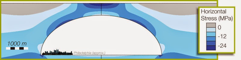
The city of Philadelphia is shown inside a theoretical lunar lava tube. A Purdue University team of researchers explored whether lava tubes more than 1 kilometer wide could remain structurally stable on the moon. Credit: Purdue University/courtesy of David Blair
Lava tubes large enough to house cities could be structurally stable on the moon, according to a theoretical study presented at the Lunar and Planetary Science Conference on March 17.
The volcanic features are an important target for future human space exploration because they could provide shelter from cosmic radiation, meteorite impacts and temperature extremes.
Lava tubes are tunnels formed from the lava flow of volcanic eruptions. The edges of the lava cool as it flows to form a pipe-like crust around the flowing river of lava. When the eruption ends and the lava flow stops, the pipe drains leave behind a hollow tunnel, said Jay Melosh, a Purdue University distinguished professor of earth, atmospheric and planetary sciences who is involved in the research.
“There has been some discussion of whether lava tubes might exist on the moon,” he said. “Some evidence, like the sinuous rilles observed on the surface, suggest that if lunar lava tubes exist they might be really big.”
Sinuous rilles are large channels visible on the lunar surface thought to be formed by lava flows. The sinuous rilles range in size up to 10 kilometers wide, and the Purdue team explored whether lava tubes of the same scale could exist.
David Blair, a graduate student in Purdue’s Department of Earth, Atmospheric and Planetary Sciences, led the study that examined whether empty lava tubes more than 1 kilometer wide could remain structurally stable on the moon.
“We found that if lunar lava tubes existed with a strong arched shape like those on Earth, they would be stable at sizes up to 5,000 meters, or several miles wide, on the moon,” Blair said. “This wouldn’t be possible on Earth, but gravity is much lower on the moon and lunar rock doesn’t have to withstand the same weathering and erosion. In theory, huge lava tubes — big enough to easily house a city — could be structurally sound on the moon.”
Blair worked with Antonio Bobet, a Purdue professor of civil engineering, and applied known information about lunar rock and the moon’s environment to civil engineering technology used to design tunnels on Earth.
The team found that a lava tube’s stability depended on the width, roof thickness and the stress state of the cooled lava, and the team modeled a range of these variables. The researchers also modeled lava tubes with walls created by lava placed in one thick layer and with lava placed in many thin layers, Blair said.
Only one other study, published in 1969, has attempted to model lunar lava tubes, he said.
In addition to Melosh, Blair and Bobet, team members include Loic Chappaz and Rohan Sood, graduate students in the School of Aeronautics and Astronautics; Kathleen Howell, Purdue’s Hsu Lo Professor of Aeronautical and Astronautical Engineering; Andy M. Freed, an associate professor of earth, atmospheric and planetary sciences; and Colleen Milbury, a postdoctoral research associate in the Department of Earth, Atmospheric and Planetary Sciences.
Note: The above story is based on materials provided by Purdue University. The original article was written by Elizabeth K. Gardner.
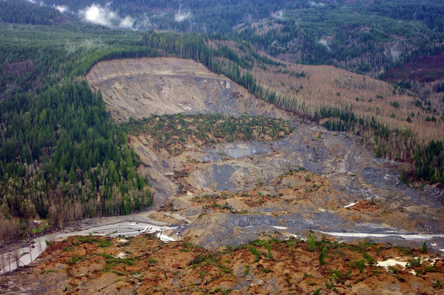
Photograph from aerial survey showing the upper parts of the landslide that occurred in northwest Washington on March 22, 2014. This photo was taken on March 27, 2014. Credit: Jonathan Godt, USGS
A landslide, also known as a landslip, is a geological phenomenon that includes a wide range of ground movements, such as rockfalls, deep failure of slopes and shallow debris flows. Landslides can occur in offshore, coastal and onshore environments. Although the action of gravity is the primary driving force for a landslide to occur, there are other contributing factors affecting the original slope stability. Typically, pre-conditional factors build up specific sub-surface conditions that make the area/slope prone to failure, whereas the actual landslide often requires a trigger before being released.
Causes of landslides
The causes of landslides are usually related to instabilities in slopes. It is usually possible to identify one or more landslide causes and one landslide trigger. The difference between these two concepts is subtle but important. The landslide causes are the reasons that a landslide occurred in that location and at that time. Landslide causes are listed in the following table, and include geological factors, morphological factors, physical factors and factors associated with human activity.
Causes may be considered to be factors that made the slope vulnerable to failure, that
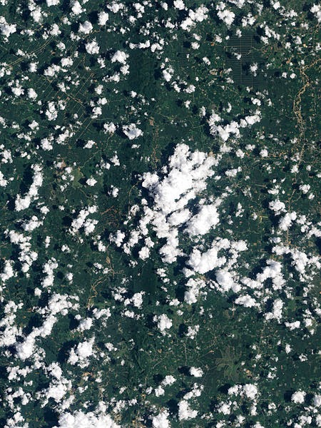
Intense rain triggered widespread landslides in southern Thailand during the last week of March 2011. Credit: NASA Earth Observatory
predispose the slope to becoming unstable. The trigger is the single event that finally initiated the landslide. Thus, causes combine to make a slope vulnerable to failure, and the trigger finally initiates the movement. Landslides can have many causes but can only have one trigger as shown in the next figure. Usually, it is relatively easy to determine the trigger after the landslide has occurred (although it is generally very difficult to determine the exact nature of landslide triggers ahead of a movement event).
Geological causes
Weathered Materials e.g. heavy rainfall
Sheared materials
Jointed or fissured materials
Adversely orientated discontinuities
Permeability contrasts
Material contrasts
Rainfall and snow fall
Earthquakes
Morphological causes
Slope angle
Uplift
Rebound
Fluvial erosion
Wave erosion
Glacial erosion
Erosion of lateral margins
Subterranean erosion
Slope loading
Vegetation change
Erosion
Physical causes
Intense rainfall
Rapid snow melt
Prolonged precipitation
Rapid drawdown
Earthquake
Volcanic eruption
Thawing
Freeze-thaw
Ground water changes
Soil pore water pressure
Surface runoff
Seismic activity
Soil erosion
Human causes
Excavation
Loading
Draw-down
Land use (e.g. construction of roads, houses etc.)
Water management
Mining
Quarrying
Vibration
Water leakage
Deforestation
Land use pattern
Pollution
Although there are multiple types of causes of landslides, the three that cause most of the damaging landslides around the world are these:
Landslides and Water
Slope saturation by water is a primary cause of landslides. This effect can occur in the form of intense rainfall, snowmelt, changes in ground-water levels, and water-level changes along coastlines, earth dams, and the banks of lakes, reservoirs, canals, and rivers.
Landsliding and flooding are closely allied because both are related to precipitation, runoff, and the saturation of ground by water. In addition, debris flows and mudflows usually occur in small, steep stream channels and often are mistaken for floods; in fact, these two events often occur simultaneously in the same area.
Landslides can cause flooding by forming landslide dams that block valleys and stream channels, allowing large amounts of water to back up. This causes backwater flooding and, if the dam fails, subsequent downstream flooding. Also, solid landslide debris can “bulk” or add volume and density to otherwise normal streamflow or cause channel blockages and diversions creating flood conditions or localized erosion. Landslides can also cause overtopping of reservoirs and/or reduced capacity of reservoirs to store water.
Landslides and Seismic Activity
Many mountainous areas that are vulnerable to landslides have also experienced at least moderate rates of earthquake occurrence in recorded times. The occurrence of earthquakes in steep landslide-prone areas greatly increases the likelihood that landslides will occur, due to ground shaking alone or shaking-caused dilation of soil materials, which allows rapid infiltration of water. The 1964 Great Alaska Earthquake caused widespread landsliding and other ground failure, which caused most of the monetary loss due to the earthquake. Other areas of the United States, such as California and the Puget Sound region in Washington, have experienced slides, lateral spreading, and other types of ground failure due to moderate to large earthquakes. Widespread rockfalls also are caused by loosening of rocks as a result of ground shaking. Worldwide, landslides caused by earthquakes kill people and damage structures at higher rates than in the United States.
Landslides and Volcanic Activity
Landslides due to volcanic activity are some of the most devastating types. Volcanic lava may melt snow at a rapid rate, causing a deluge of rock, soil, ash, and water that accelerates rapidly on the steep slopes of volcanoes, devastating anything in its path. These volcanic debris flows (also known as lahars) reach great distances, once they leave the flanks of the volcano, and can damage structures in flat areas surrounding the volcanoes. The 1980 eruption of Mount St. Helens, in Washington triggered a massive landslide on the north flank of the volcano, the largest landslide in recorded times.
Types
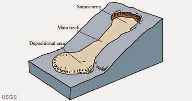
Debris flow
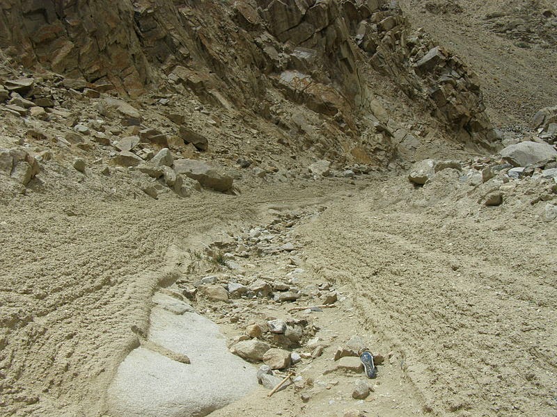
Debris flow channel with deposits left after 2010 storms in Ladakh,NW Indian Himalaya.
Slope material that becomes saturated with water may develop into a debris flow or mud flow. The resulting slurry of rock and mud may pick up trees, houses and cars, thus blocking bridges and tributaries causing flooding along its path.
Debris flow is often mistaken for flash flood, but they are entirely different processes.
Muddy-debris flows in alpine areas cause severe damage to structures and infrastructure and often claim human lives. Muddy-debris flows can start as a result of slope-related factors and shallow landslides can dam stream beds, resulting in temporary water blockage. As the impoundments fail, a “domino effect” may be created, with a remarkable growth in the volume of the flowing mass, which takes up the debris in the stream channel. The solid-liquid mixture can reach densities of up to 2 tons/m³ and velocities of up to 14 m/s (Chiarle and Luino, 1998; Arattano, 2003). These processes normally cause the first severe road interruptions, due not only to deposits accumulated on the road (from several cubic metres to hundreds of cubic metres), but in some cases to the complete removal of bridges or roadways or railways crossing the stream channel. Damage usually derives from a common underestimation of mud-debris flows: in the alpine valleys, for example, bridges are frequently destroyed by the impact force of the flow because their span is usually calculated only for a water discharge. For a small basin in the Italian Alps (area = 1.76 km²) affected by a debris flow, Chiarle and Luino (1998) estimated a peak discharge of 750 m3/s for a section located in the middle stretch of the main channel. At the same cross section, the maximum foreseeable water discharge (by HEC-1), was 19 m³/s, a value about 40 times lower than that calculated for the debris flow that occurred.
Earthflows
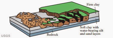
Earthflows are downslope, viscous flows of saturated, fine-grained materials, which move at any speed from slow to fast. Typically, they can move at speeds from 0.17 to 20 km/h (0.1 to 12.4 mph). Though these are a lot like mudflows, overall they are more slow moving and are covered with solid material carried along by flow from within. They are different from fluid flows because they are more rapid. Clay, fine sand and silt, and fine-grained, pyroclastic material are all susceptible to earthflows. The velocity of the earthflow is all dependent on how much water content is in the flow itself: if there is more water content in the flow, the higher the velocity will be.
These flows usually begin when the pore pressures in a fine-grained mass increase until enough of the weight of the material is supported by pore water to significantly decrease the internal shearing strength of the material. This thereby creates a bulging lobe which advances with a slow, rolling motion. As these lobes spread out, drainage of the mass increases and the margins dry out, thereby lowering the overall velocity of the flow. This process causes the flow to thicken. The bulbous variety of earthflows are not that spectacular, but they are much more common than their rapid counterparts. They develop a sag at their heads and are usually derived from the slumping at the source.
Earthflows occur much more during periods of high precipitation, which saturates the ground and adds water to the slope content. Fissures develop during the movement of clay-like material which creates the intrusion of water into the earthflows. Water then increases the pore-water pressure and reduces the shearing strength of the material.
Debris landslide
A debris slide is a type of slide characterized by the chaotic movement of rocks soil and debris mixed with water or ice (or both). They are usually triggered by the saturation of thickly vegetated slopes which results in an incoherent mixture of broken timber, smaller vegetation and other debris. Debris avalanches differ from debris slides because their movement is much more rapid. This is usually a result of lower cohesion or higher water content and commonly steeper slopes.
Steep coastal cliffs can be caused by catastrophic debris avalanches. These have been common on the submerged flanks of ocean island volcanos such as the Hawaiian Islands and the Cape Verde Islands. Another slip of this type was Storegga landslide.
Movement: Debris slides generally start with big rocks that start at the top of the slide and begin to break apart as they slide towards the bottom. This is much slower than a debris avalanche. Debris avalanches are very fast and the entire mass seems to liquefy as it slides down the slope. This is caused by a combination of saturated material, and steep slopes. As the debris moves down the slope it generally follows stream channels leaving a v-shaped scar as it moves down the hill. This differs from the more U-shaped scar of a slump. Debris avalanches can also travel well past the foot of the slope due to their tremendous speed.
Sturzstrom
A sturzstrom is a rare, poorly understood type of landslide, typically with a long run-out. Often very large, these slides are unusually mobile, flowing very far over a low angle, flat, or even slightly uphill terrain.
Shallow landslide
Lateral Spreads
Landslide in which the sliding surface is located within the soil mantle or weathered bedrock (typically to a depth from few decimetres to some metres)is called a shallow landslide. They usually include debris slides, debris flow, and failures of road cut-slopes. Landslides occurring as single large blocks of rock moving slowly down slope are sometimes called block glides.
Shallow landslides can often happen in areas that have slopes with high permeable soils on top of low permeable bottom soils. The low permeable, bottom soils trap the water in the shallower, high permeable soils creating high water pressure in the top soils. As the top soils are filled with water and become heavy, slopes can become very unstable and slide over the low permeable bottom soils. Say there is a slope with silt and sand as its top soil and bedrock as its bottom soil. During an intense rainstorm, the bedrock will keep the rain trapped in the top soils of silt and sand. As the topsoil becomes saturated and heavy, it can start to slide over the bedrock and become a shallow landslide. R. H. Campbell did a study on shallow landslides on Santa Cruz Island California. He notes that if permeability decreases with depth, a perched water table may develop in soils at intense precipitation. When pore water pressures are sufficient to reduce effective normal stress to a critical level, failure occurs.
Deep-seated landslide
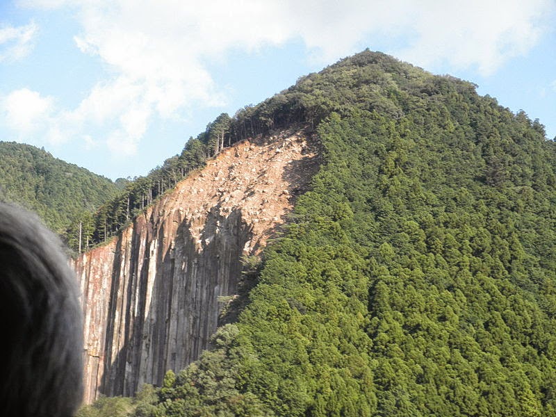
Deep-seated landslide on a mountain in Sehara, Kihō, Japan caused by torrential rain of Tropical Storm Talas
Landslides in which the sliding surface is mostly deeply located below the maximum rooting depth of trees (typically to depths greater than ten meters). Deep-seated landslides usually involve deep regolith, weathered rock, and/or bedrock and include large slope failure associated with translational, rotational, or complex movement. This type of landslides are potentially occur in an tectonic active region like Zagros Mountain in Iran. These typically move slowly, only several meters per year, but occasionally move faster. They tend to be larger than shallow landslides and form along a plane of weakness such as a fault or bedding plane. They can be visually identified by concave scarps at the top and steep areas at the toe.
Types and classification
In the following table shows a schematic landslide classification adopting the classification of Varnes 1978 and taking into account the modifications made by Cruden and Varnes, in 1996. Some integration has been made by using the definitions of Hutchinson (1988) and Hungr et al. 2001.
Type of movementType of materialBedrockEngineering soils Predominantly finePredominantly coarseFallsRockfallEarth fallDebris fallTopplesRock toppleEarth toppleDebris toppleSlidesRotational Rock slumpEarth slumpDebris slumpTranslationalFew unitsRock block slideEarth block slideDebris block slideMany unitsRock slideEarth slideDebris slideLateral spreadsRock spreadEarth spreadDebris spreadFlowsRock flowEarth flowDebris flowRock avalanche Debris avalanche(Deep creep)(Soil creep)Complex and compoundCombination in time and/or space of two or more principal types of movement
Factors Influencing Landslide Risk
Bluff Characteristics
Height: The height of a bluff can generally indicate landslide risk. While sediment strength depends on several factors, the thicker the sediment deposit, the more likely its weight will cause subsurface movement or slippage that leads to a landslide. The risk of a landslide increases when mud bluffs have a height of twenty feet or more. In general, the higher the exposed bluff face the greater the risk of a landslide.
Sediment type: Earth material that makes up a coastal bluff influences the risk of a landslide occurring. Clay and silt (muddy) sediment is the most unstable material that can make up a bluff. These fine-grained sediments are weak and prone to moving in the form of slow-motion creep, moderate-sized slumping, or large landslides. Sand and gravel deposits tend to be stronger and better drained than muddy sediment. Landslides can occur in coarse-grained bluffs although they are less frequent than muddy landslides along the Maine coast.
Slope: Coastal bluffs have a relatively steep ocean-facing slope. The angle of a bluff face varies due to factors such as the sediment type and rate of erosion at the base of the bluff. Slope is also affected by the history of slumps and landslides at the site. Some slopes are uniformly straight while others are terraced or uneven due to earth movements. In general, the steeper the slope, the easier it is for gravity to initiate a landslide.
Vegetation: Types, shapes, and distribution of vegetation above and on a bluff face can be used as an indication of site stability. In areas where the soil has shifted, either due to previous landslides or to gradual surface creep, many tree trunks can become tilted or twisted in the same direction. Curved tree trunks near the roots often indicate land movement down the face of a bluff. Large trees on the bluff face may be moved by wind and resulting root motion may loosen bluff sediment. Natural vegetation that consists only of small shrubs and trees may indicate recent bluff erosion or a landslide.
Bedrock: Crystalline rock or ledge is much more stable than any sediment bluff and not likely to erode or slide. The elevation of bedrock at the shore and inland beneath a bluff is important in determining landslide risk. Bedrock exposures along the shoreline may slow erosion and make sediment less susceptible to landsliding. Beneath a sediment bluff, bedrock may rise toward the surface and reduce the overall thickness of sediment and thus reduce the risk of deep-seated movement below the ground surface.
Natural Conditions
Waves, tides, and sea level: Several marine processes affect the risk of landslides along a coastal bluff. A gradual, but ongoing rise in sea level at a rate of about an inch per decade is causing chronic erosion along the base of many bluffs. As sea level rises, wave action and coastal flooding can reach higher and farther inland and scour more sediment from a bluff. Sea ice erodes tidal flats and the base of bluffs by abrasion and freezing sediment in ice blocks. Erosion can increase a bluff slope and make it more susceptible to landsliding. Tides are also important in washing away eroded bluff sediment which helps wave action move inland. Storms that create wind, waves, and flooding can cause more extreme erosion at the base of a bluff, increase the bluff slope, and make a landslide more likely.
Surface water: The amount, type, and location of surface water can influence bluff slope stability and may contribute to some landslides. Wetlands, ponds, and streams above the bluff can supply water to the bluff face and also to the ground water. The elevation or topography of the land surface determines which way surface water will flow. Water that runs over the face of a bluff can wash sediment to sea, increase the bluff face slope, and weaken the remaining sediment holding up the bluff. Removal of sediment from the bluff face can increase the risk of a landslide.
Ground water: Ground water inland of a bluff comes from surface sources, such as rain or a stream, uphill in the local watershed. Ground water tends to flow horizontally beneath the surface and may seep out the face of a bluff. Seeps and springs on the bluff face contribute to surface water flow and destabilize the bluff face. In addition, a high water table can saturate and weaken muddy sediment and make the ground more prone to slope failure.
Weathering: Weathering in clay and silt can change the strength of bluff sediment and stability of the bluff face. Drying of clay can increase resistance to sliding. The seasonal cycle of freezing and thawing of the bluff face can lead to slumping after a thaw.
Earthquakes: Landslides can be triggered by earthquakes. Ground vibration loosens sediment enough to reduce the strength of material supporting a bluff and a landslide results. Most landslides triggered by earthquakes in sediment like that found in Maine have been of Richter magnitude 5 or more. These are relatively rare events, but a few have occurred in historical time.
Human Activity
Land use: Human activity and land use may contribute to or reduce the risk of a landslide. Actions that increase surface water flow to a bluff face, watering lawns or grading slopes, add to natural processes destabilizing the bluff face. Surface water, collected by roofs, driveways, paths, and lawns flows toward and down the bluff face. Walkways down the face of a bluff can lead to greater erosion from foot traffic or the concentration of surface water flow. Both surface and ground water above a bluff can be supplied by pipes, culverts, surface drains, and septic systems. Increased water below ground can weaken a bluff and contribute to internal weakness that leads to a landslide. Greater seepage of water out of the bluff face can also increase the risk.
Clearing of vegetation from the bluff face can lead to greater bluff erosion and a steeper bluff that is more prone to landslide. Vegetation tends to remove ground water, strengthen soil with roots, and lessen the impact of heavy rain on the bluff face.
Adding weight to the top of a bluff can increase the risk of a landslide. Buildings, landscaping, or fill on the top of the bluff can increase the forces that result in a landslide. Saturating the ground with water that raises the water table also adds weight. Even ground vibration, such as well drilling or deep excavation, may locally increase the risk of a landslide.
Shoreline engineering in the form of seawalls, rip rap, or other solid structures is sometimes used to reduce wave erosion at the toe of a bluff. In some settings, engineering can increase the rate of beach or tidal flat erosion and lower the shore profile over time. This intertidal erosion can undermine engineering and result in less physical support of the base of the bluff by natural sediment. Where engineering ends along a shore, erosion can become worse on adjacent properties. Engineering alone cannot prevent some large landslides.
In general, human activities that increase the amount or rate of natural processes may, in various ways, contribute to landslide risk.
The Bay Area fault system and the spot (red star) where the Hayward Fault branches off from the Calaveras Fault. The white lines indicate faults recognized by the USGS. The red line is the newly discovered surface trace connecting the southern end of the Hayward Fault to the Calaveras Fault, once thought to be an independent system. The surface trace is offset by several kilometers from the deep portion of the fault 3-5 km below ground (blue line). Credit: Estelle Chaussard, UC Berkeley
University of California, Berkeley seismologists have proven that the Hayward Fault is essentially a branch of the Calaveras Fault that runs east of San Jose, which means that both could rupture together, resulting in a significantly more destructive earthquake than previously thought.
“The maximum earthquake on a fault is proportional to its length, so by having the two directly connected, we can have a rupture propagating across from one to the other, making a larger quake,” said lead researcher Estelle Chaussard, a postdoctoral fellow in the Berkeley Seismological Laboratory. “People have been looking for evidence of this for a long time, but only now do we have the data to prove it.”
The 70-kilometer-long Hayward Fault is already known as one of the most dangerous in the country because it runs through large population areas from its northern limit on San Pablo Bay at Richmond to its southern end south of Fremont.
In an update of seismic hazards last month, the U.S. Geological Survey estimated a 14.3 percent likelihood of a magnitude 6.7 or greater earthquake on the Hayward Fault in the next 30 years, and a 7.4 percent chance on the Calaveras Fault.
These are based on the assumption that the two faults are independent systems, and that the maximum quake on the Hayward Fault would be between magnitudes 6.9 and 7.0. Given that the Hayward and Calaveras faults are connected, the energy released in a simultaneous rupture could be 2.5 times greater, or a magnitude 7.3 quake.
“A rupture from Richmond to Gilroy would produce about a 7.3 magnitude quake, but it would be even greater if the rupture extended south to Hollister, where the Calaveras Fault meets the San Andreas Fault,” Chaussard said.
Chaussard and her colleagues, including Roland Bürgmann, a UC Berkeley professor of earth and planetary science, reported their findings in the journal Geophysical Research Letters.
Creep connects two faults
Chaussard said there has always been ambiguity about whether the two faults are connected. The Hayward Fault ends just short of the Calaveras Fault, which runs about 123 kilometers from north of Danville south to Hollister in the Salinas Valley.
The UC Berkeley team used 19 years of satellite data to map ground deformation using interferometric synthetic aperture radar (InSAR) and measure creep along the southern end of the Hayward Fault, and found, surprisingly, that the creep didn’t stop south of Fremont, the presumed southern end of the fault, but continued as far as the Calaveras Fault.
“We found that it continued on another 15 kilometers and that the trace merged with the trace of the Calaveras Fault,” she said. In addition, seismic data show that micro-earthquakes on these faults 3-5 kilometers underground also merge. “With this evidence from surface creep and seismicity, we can argue for a direct junction on the surface and at depth for the two faults.”
Both are strike-slip faults — the western side moves northward relative to the eastern side. The researchers found that the underground portion of the Hayward Fault meets the Calaveras Fault 10 kilometers farther north than where the creeping surface traces of both faults meet. This geometry implies that the Hayward Fault dips at an angle where it meets the Calaveras Fault.
InSAR revolutionizes mapping
Chaussard said that the many years of InSAR data, in particular from the European Space Agency’s ERS and Envisat satellites from 1992 to 2011, were critical to connecting the two faults.
Creep, or the surface movement along a fault, is evidenced by offset curbs, streets and home foundations. It is normally determined by measuring points on opposite sides of a fault every few years, but that is hard to do along an entire fault or in difficult terrain. InSAR provides data over large areas even in vegetated terrains and outside of urban areas, and with the repeated measurements over many years InSAR can detect deformation with a precision of 2 millimeters per year.
“With InSAR, we have access to much larger spatial coverage,” said Chaussard, who has been expanding the use of InSAR to measure water resources and now ground deformation that occurs between earthquakes. “Instead of having a few points, we have over 200,000 points in the Bay Area. And we have access to areas we couldn’t go to on the ground.”
She noted that while creep relieves stress on a fault gradually, eventually the surface movement must catch up with the long-term underground fault movement. The Hayward Fault moves at about 10 millimeters per year underground, but it creeps at only 3 to 8 millimeters per year. Earthquakes occur when the surface suddenly catches up with a fault’s underground long-term movement.
“Creep is delaying the accumulation of stress needed to get to an earthquake, but it does not cancel the earthquake,” Chaussard said.
Reference:
E. Chaussard, R. Bürgmann, H. Fattahi, R. M. Nadeau, T. Taira, C. W. Johnson, I. Johanson. Potential for larger earthquakes in the East San Francisco Bay Area due to the direct connection between the Hayward and Calaveras Faults. Geophysical Research Letters, 2015; DOI: 10.1002/2015GL063575
Simulation of the Deepwater Horizon blowout based on oil-in-water experimental data: distribution of oil mass in the water column? at day 60, assuming no injection of dispersant at the wellhead. We note that the highest oil concentration (red) remain at depth. Diluted oil by 5-25 folds, reaches the surface as far as 200 km downstream from the response zone of the accident. Credit: C-IMAGE
A first-of-its-kind study observed how oil droplets are formed and measured their size under high pressure. They further simulated how the atomized oil spewing from the Macondo well reached the ocean’s surface during the Deepwater Horizon accident. The findings from the University of Miami (UM) Rosenstiel School of Marine and Atmospheric Science and University of Western Australia research team suggest that the physical properties in deep water create a natural dispersion mechanism for oil droplets that generates a similar effect to the application of chemical dispersants at oil spill source.
“These results support our initial modeling work that the use of toxic dispersants at depth should not be a systematic oil spill response,” said Claire Paris, Associate Professor of Ocean Sciences at the UM Rosenstiel School. “It could very well be unnecessary in some cases.”
The research team from C-IMAGE (Center for the Integrated Modeling and Analysis of the Gulf Ecosystem) conducted eight experiments to simulate different pressures of oil from a blowout at depth. The oil was placed in a high-pressure chamber, called a sapphire autoclave, and monitored using a high-speed, high-resolution camera to evaluate how droplets form at varying turbulent conditions.
“This is the first time that we’ve been able to visually monitor how droplets break up and coalesce at up to 120 times atmospheric pressure,” said Zachary Aman, associate professor of mechanical and chemical engineering at the University of Western Australia. “When paired with the high pressures and flow rates of Macondo, the results suggest a natural mechanism by which oil is dispersed into small droplets.”
The results of the laboratory experiment were applied in a field-scale simulation under the same physical conditions that existed during the Macondo well blowout. In the computer simulation, the team tracked the oil released at a constant rate of 1000 oil droplets every two hours at a depth of 300 meters above the Macondo well, corresponding to the depth of the observed deep plume, from April 20 to July 15, 2010, when the Macondo well was capped; droplets were tracked for an additional 24 days after the cap was in place.
Based on the experimental data and modelling, the researchers suggest that the use of chemical dispersants may have reduced the mean oil droplet diameter from about 80 to 45 µm, which would have reduced the amount of oil reaching the surface only by up to 3%. The model simulations showed that if the blowout occurred in shallow water conditions, or at a smaller rate of hydrocarbon release, dispersant may have had a more significant impact on the oil flowing from the well.
The research paper, entitled “High-pressure visual experimental studies of oil-in-water dispersion droplet size,” will be published in the May 4 edition of the journal Chemical Engineering Science and is currently available in the online edition. The study’s co-author’s include Claire B. Paris and David Lindo-Atichati of the UM Rosenstiel School and Zachary Aman, Eric F. May and Michael L. Johns of the University of Western Australia.
Reference:
Zachary M. Aman, Claire B. Paris, Eric F. May, Michael L. Johns, David Lindo-Atichati. High-pressure visual experimental studies of oil-in-water dispersion droplet size. Chemical Engineering Science, 2015; 127: 392 DOI: 10.1016/j.ces.2015.01.058
Backscattered electron image of Hyperammina deformis. Credit: Courtesy Merlynd and Galina Nestell
A new study led by scientists with The University of Texas at Arlington demonstrates for the first time how elemental carbon became an important construction material of some forms of ocean life after one of the greatest mass extinctions in the history of Earth more than 252 million years ago.
As the Permian Period of the Paleozoic Era ended and the Triassic Period of the Mesozoic Era began, more than 90 percent of terrestrial and marine species became extinct. Various proposals have been suggested for this extinction event, including extensive volcanic activity, global heating, or even one or more extraterrestrial impacts.
The work is explained in the paper, “High influx of carbon in walls of agglutinated foraminifers during the Permian-Triassic transition in global oceans,” which is published in the March edition of International Geology Review.
Researchers focused on a section of the latest Permian aged rocks in Vietnam, just south of the Chinese border, where closely spaced samples were collected and studied from about a four-meter interval in the boundary strata.
Merlynd Nestell, professor of earth and environmental sciences in the UT Arlington College of Science and a co-author of the paper, said there was extensive volcanic activity in both the Northern and the Southern Hemispheres during the Permian-Triassic transition.
“Much of the volcanic activity was connected with the extensive Siberian flood basalt known as the Siberian Traps that emerged through Permian aged coal deposits and, of course, the burning of coal created CO2,” Nestell said.
He noted that there was also synchronous volcanic activity in what is now Australia and southern China that could have burned Permian vegetation. The carbon from ash accumulated in the atmosphere and marine environment and was used by some marine microorganisms in the construction of their shells, something they had not done before.
This new discovery documents elemental carbon as being a major construction component of the tiny shells of single-celled agglutinated foraminifers, ostracodes, and worm tubes that made up part of the very limited population of bottom-dwelling marine organisms surviving the extinction event.
“Specimens of the boundary interval foraminifers seen in slices of rock that were ground thin and studied from other places in the world revealed black layers,” said Galina P. Nestell, study co-author and adjunct research professor of earth and environmental sciences at UT Arlington. “But nobody really checked the composition of the black material.”
Nestell said this phenomenon has never been reported although sequences of rocks that cross this important Permian-Triassic boundary have been studied in Iran, Hungary, China, Turkey, Slovenia and many other parts of the world.
For the study, Asish Basu, chair of earth and environmental sciences at UT Arlington, analyzed clusters of iron pyrite attached to the walls of the foraminifer shells for lead isotopes. Data from these pyrite clusters support the presence of products of coal combustion that contributed to the high input of carbon into the marine environment immediately after the extinction event.
Brooks Ellwood, emeritus professor of Earth and Environmental Sciences at UT Arlington and a professor in the Louisiana State University Department of Geology and Geophysics, collected the samples to study the Permian-Triassic boundary interval using magnetic and geochemical properties. He and his colleague Luu Thi Phuong Lan of the Vietnamese Academy of Science and Technology in Hanoi, Vietnam, also collected the samples used in the biostratigraphic work by the Nestells and Bruce Wardlaw of the Eastern Geology and Paleoclimate Science Center at the U.S. Geological Survey and adjunct professor at UT Arlington.
By using time-series analysis of magnetic measurements, Ellwood discovered the extinction event to have lasted about 28,000 years. It ended about 91,000 years before the actual Permian-Triassic boundary level — as defined worldwide by the first appearance of the fossil conodont species Hindeodus parvus — identification done by Wardlaw.
Galina Nestell said the high carbon levels began after the extinction event about 82,000 years before the official boundary horizon and continued until about 3,000 years after the Permian-Triassic boundary horizon. The boundary horizon is calculated to be 252.2 million years before present.
Other co-authors who contributed to parts of the study include Andrew Hunt, EES associate professor at UT Arlington, Nilotpal Ghosh of the University of Rochester; Harry Rowe of the Bureau of Economic Geology at the University of Texas at Austin; Jonathan Tomkin of the University of Illinois, Urbana; and Kenneth Ratcliffe of Chemostrat Inc. in Houston.
Reference:
Galina P. Nestell, Merlynd K. Nestell, Brooks B. Ellwood, Bruce R. Wardlaw, Asish R. Basu, Nilotpal Ghosh, Luu Thi Phuong Lan, Harry D. Rowe, Andrew Hunt, Jonathan H. Tomkin, Kenneth T. Ratcliffe. High influx of carbon in walls of agglutinated foraminifers during the Permian–Triassic transition in global oceans. International Geology Review, 2015; 57 (4): 411 DOI: 10.1080/00206814.2015.1010610
Artist’s conception of an oviraptor using its tail feathers in a mating display. Credit: Sydney Mohr
Paleontologists at the University of Alberta have discovered evidence of a prehistoric romance and the secret to sexing some dinosaurs.
“Determining a dinosaur’s gender is really hard,” says graduate student Scott Persons, lead author of the research. “Because soft anatomy seldom fossilizes, a dinosaur fossil usually provides no direct evidence of whether it was a male or a female.”
Instead, the new research focuses on indirect evidence. Modern birds, the living descendants of dinosaurs, frequently show sexually dimorphic display structures. Such structures—like the fans of peacocks, the tall crests of roosters or the long tail feathers of some birds of paradise—are used to attract and court mates, and are almost always much larger in males (who do the courting) than in females (who do the choosing).
Back in 2011, Persons and his colleagues published research on the tails of a group of birdlike dinosaurs called oviraptors. Oviraptors were strictly land-bound animals, but according to the study, they possessed fans of long feathers on the ends of their tails. If these dinosaurs weren’t able to fly, what good were their tail feathers?
“Our theory,” explains Persons, “was that these large feather fans were used for the same purpose as the feather fans of many modern ground birds, like turkeys, peacocks and prairie chickens: they were used to enhance courtship displays. My analysis of the tail skeletons supported this theory, because the skeletons showed adaptations for both high tail flexibility and enlarged tail musculature—both traits that would have helped an oviraptor to flaunt its tail fan in a mating dance.”
The U of A researchers took the idea a step further. “The greatest test of any scientific theory is its predictive power,” says Persons. “If we were right, and oviraptors really were using their tail fans to court mates, then, just as in modern birds, the display structures ought to be sexually dimorphic. We published the prediction that careful analysis of more oviraptor tails would reveal male and female differences within the same species.”
That prediction has come home to roost. In the new study, published this week in the journal Scientific Reports, Persons and his team have confirmed sexual dimorphism, after meticulous observation of two oviraptor specimens. The two raptors were discovered in the Gobi Desert of Mongolia. Both died and were buried next to each other when a large sand dune collapsed on top of them.
When they were first unearthed, the two oviraptors were given the nicknames “Romeo and Juliet,” because they seemed reminiscent of Shakespeare’s famously doomed lovers. It turns out that the nickname may have been entirely appropriate.
“We discovered that, although both oviraptors were roughly the same size, the same age and otherwise identical in all anatomical regards, ‘Romeo’ had larger and specially shaped tail bones,” says Persons. “This indicates that it had a greater capacity for courtship displays and was likely a male.” By comparison, the second specimen, “Juliet,” had shorter and simpler tail bones, suggesting a lesser capacity for peacocking, and has been interpreted as a female.
According to Persons, the two may very well have been a mated pair, making for an altogether romantic story, as the dinosaur couple was preserved side by side for more than 75 million years.
Reference:
“A possible instance of sexual dimorphism in the tails of two oviraptorosaur dinosaurs.” Scientific Reports 5, Article number: 9472 DOI: 10.1038/srep09472