

Seismic Tomography: Visualizing Density Anomalies in the Lower Mantle
Seismic tomography is the primary geophysical method used to image the internal structure of the Earth by analyzing variations in seismic wave speeds. In the lower mantle—extending from ~660 km depth to the core–mantle boundary at 2,890 km—seismic tomography has revolutionized our understanding of density anomalies, subducted slabs, mantle plumes, and large low-shear-velocity provinces (LLSVPs).
By converting global seismic travel-time data into three-dimensional velocity models, geophysicists can infer temperature variations, compositional heterogeneities, and dynamic mantle flow patterns. Although seismic tomography does not measure density directly, velocity anomalies provide powerful proxies for interpreting deep Earth structure.
Understanding how seismic tomography works—and what it reveals about lower mantle dynamics—is essential for students and geologists investigating mantle convection, plate tectonics, and planetary evolution.
What Is Seismic Tomography? A Definition
Basic Principle
Seismic tomography is analogous to medical CT scanning. Just as X-rays travel at different speeds through tissues of varying density, seismic waves travel at different velocities through rocks depending on their temperature, composition, and phase state.
By analyzing:
- Travel times of P-waves and S-waves
- Waveform distortions
- Amplitude variations
scientists reconstruct 3D velocity structures inside the Earth.
Seismic Wave Types Used in Tomography
P-Waves (Primary Waves)
- Compressional waves
- Travel through solids and liquids
- Sensitive to both elastic modulus and density
S-Waves (Shear Waves)
- Travel only through solids
- Particularly sensitive to shear modulus
- Most useful for imaging lower mantle structure
In lower mantle studies, shear-wave velocity (Vs) anomalies are especially important because they respond strongly to temperature and compositional variations.
From Velocity Anomalies to Density Anomalies
Velocity–Density Relationship
Seismic tomography measures velocity, not density directly. However, mineral physics provides relationships linking:
- Seismic velocity
- Temperature
- Composition
- Elastic moduli
- Density
Higher temperatures generally reduce seismic velocities and density, while colder, subducted slabs increase both.
Thermal vs Compositional Effects
Velocity anomalies may result from:
- Thermal variations
– Hot mantle → low velocity → lower density
– Cold slabs → high velocity → higher density - Compositional heterogeneity
– Recycled oceanic crust
– Iron-rich regions
– Primordial reservoirs
Distinguishing between these causes is a central challenge in interpreting lower mantle tomography.
Structure of the Lower Mantle Revealed by Seismic Tomography
Subducted Slabs Penetrating the Lower Mantle
High-velocity anomalies beneath subduction zones correspond to cold, dense slabs descending into the lower mantle. Tomographic models reveal slabs penetrating to depths of 1,000–2,000 km and sometimes reaching the core–mantle boundary.
This confirms that:
- Subduction is a whole-mantle process.
- Cold lithosphere can survive transit through phase transitions at 660 km.
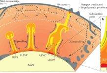
Large Low-Shear-Velocity Provinces (LLSVPs)
Two enormous low-velocity regions dominate the base of the mantle beneath Africa and the Pacific.
These LLSVPs are:
- 1–3% slower in shear velocity
- Thousands of kilometers across
- Likely thermochemical structures
Their margins appear to be preferred sites for mantle plume initiation.
Mantle Plumes
Narrow, low-velocity columns rising from deep mantle regions are interpreted as mantle plumes feeding hotspots such as Hawaii and Iceland.
Although resolution decreases with depth, modern tomography supports plume-like upwellings extending from near the core–mantle boundary to the lithosphere.
Methods of Seismic Tomography
Global Travel-Time Tomography
Uses millions of travel-time measurements from global earthquakes. Provides large-scale images of mantle structure.
Finite-Frequency Tomography
Accounts for wavefront sensitivity, improving resolution compared to ray-theory approaches.
Full-Waveform Inversion
Uses entire seismic waveforms rather than only travel times, producing higher-resolution models of deep mantle structure.
These advances have dramatically improved imaging of lower mantle density anomalies.
Resolution and Limitations of Seismic Tomography
Resolution Constraints
Resolution depends on:
- Earthquake distribution
- Seismic station coverage
- Wave frequency
- Inversion method
Lower mantle imaging remains less resolved than upper mantle imaging.
Trade-Off Between Temperature and Composition
Because both temperature and composition affect velocity, interpretations require integration with:
- Geodynamic modeling
- Mineral physics experiments
- Geochemical constraints
Tomography alone cannot uniquely determine density variations.
Implications for Mantle Convection and Geodynamics
Whole-Mantle Convection
Tomography supports models of whole-mantle convection, with:
- Cold slabs descending
- Hot plumes rising
- Long-wavelength circulation patterns
Core–Mantle Boundary Dynamics
Low-velocity regions near the core–mantle boundary influence:
- Heat flux from the core
- Geodynamo behavior
- Long-term mantle evolution
Understanding density anomalies in the lower mantle is therefore essential for modeling Earth’s thermal history.
Seismic Tomography and Plate Tectonics
Tomographic images show that present-day subduction zones correlate with deep mantle structures, linking surface tectonics to deep interior processes.
This reinforces the concept that:
- Plate tectonics is dynamically coupled to mantle convection.
- Surface geology reflects deep mantle heterogeneity.
Future Directions in Lower Mantle Imaging
Advances expected in the coming decades include:
- Higher-density global seismic networks
- Ocean-bottom seismology expansion
- Machine-learning-assisted inversions
- Integrated mineral physics–geodynamics models
These developments will refine our understanding of lower mantle density anomalies and their role in Earth evolution.
References
- Dziewonski, A. M. (1984). Mapping the lower mantle: Determination of lateral heterogeneity. Journal of Geophysical Research, 89, 5929–5952.
- Romanowicz, B. (2003). Global mantle tomography. Science, 301, 1884–1888.
- Ritsema, J., Deuss, A., van Heijst, H. J., & Woodhouse, J. H. (2011). S40RTS global seismic model. Geophysical Journal International, 184, 1223–1236.
- Garnero, E. J., McNamara, A. K., & Shim, S.-H. (2016). Continent-sized anomalous zones in the lower mantle. Nature Geoscience, 9, 481–489.
- Li, C., van der Hilst, R. D., & Engdahl, E. R. (2008). A new global model of P-wave speed variation in Earth’s mantle. Geochemistry, Geophysics, Geosystems, 9, Q05018.
- French, S. W., & Romanowicz, B. (2014). Whole-mantle radially anisotropic tomography. Nature, 525, 95–99.