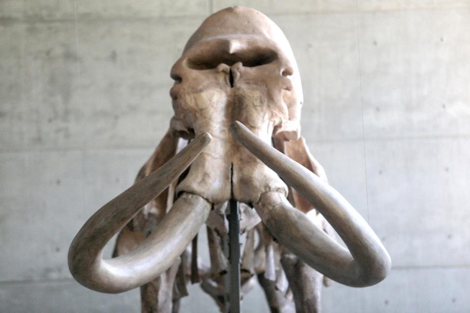
A well-preserved skeleton of a mammoth — a prehistoric creature that roamed the Earth for millions of years before dying out 5,000 years ago Credit: AFP Photo/Pedro Pardo
Mammoth remains that could be around 20,000 years old have been discovered at a building site in central Switzerland, a local official said Friday.
“It’s a very exciting discovery, because the last mammoth find (in the canton of Zug) was 50 years ago,” said Renata Huber of the canton’s heritage and archaeological department.
During the construction of an office building in the town of Rotkreuz late last month, a heavy digger emerged from the ground lifting what appeared to be a large tusk, Huber said.
Local government specialists were immediately called in, and several other bones were later discovered, but not enough to reconstruct a full mammoth, she added.
“It’s not clear if this is all one animal,” Huber said, noting that the find was not as significant as those previously unearthed in Zurich, which enabled specialists to recreate an entire carcass.
Experts will now try to date the remains, and specialists will stay at the construction site until they are satisfied that there are no further bones to be uncovered.
The discovery is unlikely to shed any new light on the type of prehistoric species that once lived on what is now Swiss land, but Huber said the significance of the find should not be understated.
“For an archaeologist, this is a once in a lifetime thing.”
Note: The above post is reprinted from materials provided by AFP.
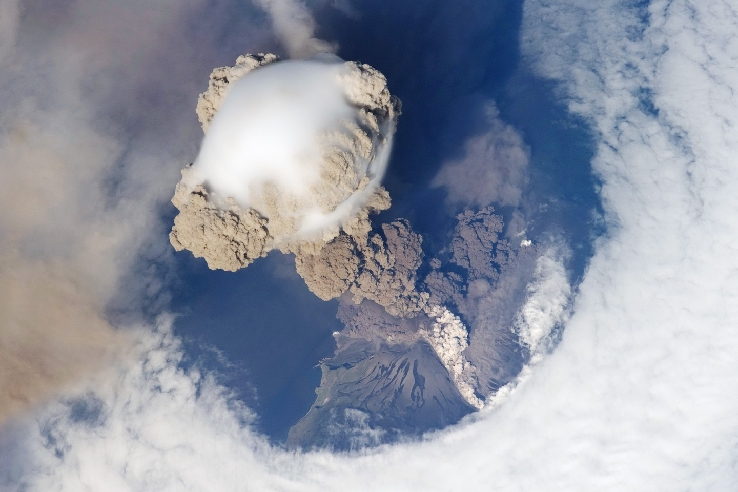
This is a plume of ash from the Sarychev volcano in the Kuril islands, northeast of Japan. The picture was taken from the International Space Station during the early stage of the volcano’s eruption on June 12, 2009. Credit: NASA
In June, 1991, Mount Pinatubo in the Philippines exploded, blasting millions of tons of ash and gas over 20 miles high – deep into the stratosphere, a stable layer of our atmosphere above most of the clouds and weather. Certain gases in the massive plume from this volcano acted like a sunshield by scattering some of the sun’s light, preventing it from reaching the surface and causing average surface temperatures to drop worldwide by an estimated 0.5 degrees Celsius (0.9 degrees Fahrenheit).
“We’ve been trying to better understand how volcanoes alter the climate for about 30 years now,” said Lori Glaze of NASA’s Goddard Space Flight Center in Greenbelt, Maryland. “The Mount Saint Helens eruption in 1980 (Washington state) and the El Chichon eruption in 1982 (Mexico) were both similar-sized eruptions. There wasn’t much of a climate effect after Mount Saint Helens, but after El Chichon, there was a big global cooling event for a couple years.”
“We didn’t understand why, so people started looking into that and it turned out that the El Chichon eruption included much more sulfur than Mount Saint Helens,” said Glaze.
The eruptions of El Chichon and Pinatubo were powerful enough to propel their gases into the stratosphere, which gave them the potential to alter short-term climate. “Since the stratosphere is stable, if gas in volcanic plumes gets into the stratosphere, it stays there for a long time – a couple years,” said Glaze. “Although there are many complications, the bottom line is that when these gases produce aerosols in the stratosphere, they scatter some of the sun’s radiation, which warms the stratosphere and causes a net cooling at the surface. The gas in these volcanic plumes – primarily sulfur dioxide (SO2) and hydrogen sulfide (H2S) – which doesn’t come out in large amounts—reacts to form a layer of sulfuric acid (H2SO4) in the stratosphere. This layer scatters some of the sun’s infrared radiation.”
Another type of volcano called a “flood-basalt eruption” doesn’t explode as dramatically, but dwarfs these examples with much bigger volumes of gas and lava erupted. “With eruptions like Pinatubo, you get one shot of sulfur dioxide and other gases into the stratosphere, but then the volcano is quiet for hundreds or thousands of years,” said Glaze. “With a flood-basalt eruption, you’re repeatedly ejecting these chemicals into the atmosphere over tens, hundreds, or maybe even thousands of years. Each eruption itself may not be the biggest thing you’ve ever seen, but you’re continuously supplying gas to the atmosphere over a long period time.”
There haven’t been any flood-basalt volcanic eruptions in human history, which is probably a good thing. “It’s almost unfathomable how big these lava flows are,” said Glaze. “A large part of the western part of the state of Washington is covered in 1.5 kilometers-thick (thousands of yards) lava from the Columbia River flood-basalt eruptions.” One eruption of the Columbia River basalt formation, the Roza eruption, is the focus of Glaze and her team’s analysis. It happened about 14.7 million years ago and produced about 1,300 cubic kilometers (over 300 cubic miles) of lava over an estimated period of ten to fifteen years.
Although flood-basalt eruptions were enormous, they were not as explosive as eruptions like Pinatubo. The molten rock (magma) in flood-basalt eruptions flowed easily. This allowed gas that was trapped in it to be released easily as well. This magma produces “fire-fountain” eruptions – a fountain of lava rising hundreds of meters (hundreds of yards) into the air. Often these eruptions begin along a crack in the Earth, called a fissure, up to several kilometers (a few miles) long, producing a dramatic glowing curtain of lava. Fire-fountain eruptions are seen on a smaller scale today in places like Hawaii and Mount Etna in Sicily, Italy.
The magma that powers Pinatubo-type eruptions is thicker, and flows more slowly. Gas dissolved in this thick magma can’t escape as easily, so when pressure is suddenly released at the beginning of these eruptions, it’s like popping the cork on a bottle of champagne – all the gas rushes out at once, producing an explosive eruption.
Since “fire-fountain” eruptions aren’t as explosive, scientists wonder whether the gases from them are propelled high enough to reach the stratosphere, allowing the very large fire-fountain eruptions that produced the flood basalts to potentially alter the climate. The answer depends not only on how vigorous the eruption is – taller fire fountains produce higher gas plumes – but also on where the stratosphere begins.
The boundary between the unstable lower atmosphere (troposphere) and the stable stratosphere is called the tropopause. Because warmer air expands more and rises higher than cooler air, the tropopause is highest over the equator and gradually becomes lower until it reaches its minimum height over the poles. Thus a fire-fountain plume from a volcano at high latitudes near the polar-regions has a better chance of reaching the stratosphere than one from a volcano near the equator.
The height of the boundary has also changed over time, as the contents of the atmosphere have changed. For example, carbon dioxide gas traps heat from the sun, so when there was more carbon dioxide in the atmosphere, temperatures were warmer and the tropopause was higher.
The question of whether large fire-fountain eruptions can change climate was raised by a similar but much smaller-scale fire-fountain eruption in Iceland, according to Glaze. “The Laki eruption in 1783 to 1784 injected sulfur dioxide into the upper troposphere and lower stratosphere through repeated eruptions over a period of eight months, affecting climate in the northern hemisphere during 1783 and possibly through 1784,” said Glaze. Ben Franklin, living in France at the time, noticed the haze and severe winter and speculated on whether Icelandic volcanoes could have changed the weather, according to Glaze.
To answer this question, Glaze and her team applied a computer model they developed to calculate how high volcanic plumes rise. “This is the first time a model like this has been used to calculate whether the plume of ash and gas above a large fire-fountain volcano like the Roza eruption could reach the stratosphere at the time and location of the event,” said Glaze.
Her team estimated the tropopause height given the eruption’s latitude (about 45 degrees North) and the contents of the atmosphere at the time of the eruption and found that the eruption could have reached the stratosphere. Glaze is lead author of a paper on this research published August 6 in the journal Earth and Planetary Science Letters.
“Assuming five-kilometer-long (3.1 mile-long) active fissure segments, the approximately 180 kilometers (about 112 miles) of known Roza fissure length could have supported about 36 explosive events or phases over a period of maybe ten to fifteen years, each with a duration of three to four days,” said Glaze. “Each segment could inject as much as 62 million metric tons per day of sulfur dioxide into the stratosphere while actively fountaining, the equivalent of about three Pinatubo eruptions per day.”
The team verified their model by applying it to the 1986 Izu-Oshima eruption, a well-documented eruption in Japan that produced spectacular fire fountains 1.6 kilometers (almost a mile) high. “This eruption produced observed maximum plume heights of 12 to 16 km (7.4 to 9.9 miles) above sea level,” said Glaze. When the team input fountain height, temperature, fissure width, and other characteristics similar to the Izu-Oshima eruption into their model, it predicted maximum plume heights of 13.1 to 17.4 km (8.1 to 10.8 miles), encompassing most of the observed values.
“Assuming the much larger Roza eruption could sustain fire-fountain heights similar to Izu-Oshima, our model shows that Roza could have sustained buoyant ash and gas plumes that extended into the stratosphere at about 45 degrees north,” said Glaze.
Although the team’s research suggests the Roza eruption had the potential to alter climate, scientists still have to search for evidence of a climate change around the time of the eruption, perhaps an extinction event in the fossil record, or indications of changes in atmospheric chemistry or sea levels, according to Glaze.
“For my personal research, I would like to take these results and look at some of the really large ancient fissure eruptions on Venus and Mars,” said Glaze. “There are other gases in volcanic plumes like water vapor and carbon dioxide. These gases don’t have significant effect on Earth because there is so much in the atmosphere already. However, on Venus and Mars, the effect of water vapor becomes very important because there is so little of it in their atmospheres. Venus is one of my favorite places to study and I want to ask if there was active volcanism on Venus today, what should we be looking for?”
The surface of Venus is hidden under a thick cloud layer, so a volcanic plume might not be visible from space, but there is the possibility that an active volcano could produce noticeable changes in atmospheric chemistry.
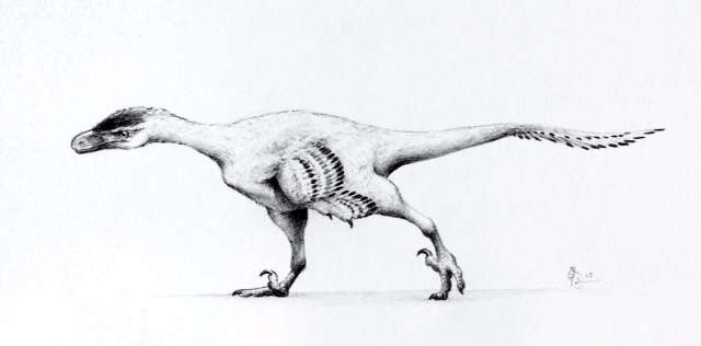
Artist’s rendering of small theropod from the South Pyrenees. Credit: Sydney Mohr (artist), University of Alberta.
Researchers have examined one of the smallest parts of the fossil record—theropod teeth—to shed light on the evolution of dinosaurs at the end of the Cretaceous. Findings published in the prestigious journal Acta Palaeontologica Polonica have effectively quadrupled the dinosaur diversity in the area of study, eight localities from Treviño County, Huesca and Lerida—including the exceptional site of Laño. There were previously only two known species in the area.
Artist’s rendering of small dromaeosaur from the South Pyrenees. Credit: Sydney Mohr (artist), University of Alberta
The study of 142 isolated teeth from the Campanian-Maastrichtian of the South Pyrenean Basin suggests six additional species of toothed theropods (five small, one large) were present in the region. “Studying these small parts helps us reconstruct the ancient world where dinosaurs lived and to understand how their extinction happened,” says lead author Angelica Torices, post-doctoral fellow in biological sciences at the University of Alberta. “Teeth are especially important in the study of Upper Cretaceous creatures in Spain and the rest of Europe because we don’t have complete skeletons of theropods from that time in those locations. We have to rely on these small elements to reconstruct the evolution of these dinosaurs, particularly the theropods.”
Carnivorous dinosaurs replaced their teeth continuously, with just one dinosaur producing a huge number of these dental pieces and an endless number of clues for understanding these mysterious creatures. This study demonstrates the value of isolated teeth in reconstructing the composition of dinosaur paleofaunas when other, more complete material is not present, allowing interpretation of the evolution of diversity through time.
The findings provide huge strides in understanding not only the diversity of carnivorous dinosaurs at the end of the Cretaceous in Europe, but also how the diversity of large animals responds to climatic changes. “It completely changes the vision of the ecosystem,” says Torices. “Moreover, we now understand that these dinosaurs disappeared very quickly in geological time, probably in a catastrophic event. Climatic models show that we may reach Cretaceous temperatures within the next century, and the only way we can study biodiversity under such conditions is through the fossil record.”
Reference:
“Theropod dinosaurs from the Upper Cretaceous of the South Pyrenees Basin on Spain” appeared in Acta Palaeontologica Polonica in August, 2015. DOI: 10.4202/app.2012.0121
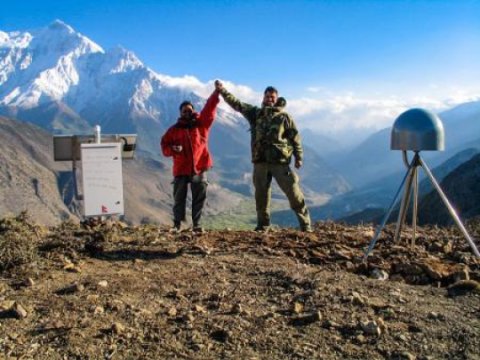
John Galetzka, then of Caltech, and Sudhir Rajaure, of the Department of Mines and Geology in Kathmandu, install a high-rate GPS station in the Himalaya. Credit: John Galetzka
For more than 20 years, Caltech geologist Jean-Philippe Avouac has collaborated with the Department of Mines and Geology of Nepal to study the Himalayas–the most active, above-water mountain range on Earth–to learn more about the processes that build mountains and trigger earthquakes. Over that period, he and his colleagues have installed a network of GPS stations in Nepal that allows them to monitor the way Earth’s crust moves during and in between earthquakes. So when he heard on April 25 that a magnitude 7.8 earthquake had struck near Gorkha, Nepal, not far from Kathmandu, he thought he knew what to expect–utter devastation throughout Kathmandu and a death toll in the hundreds of thousands.
“At first when I saw the news trickling in from Kathmandu, I thought there was a problem of communication, that we weren’t hearing the full extent of the damage,” says Avouac, Caltech’s Earle C. Anthony Professor of Geology. “As it turns out, there was little damage to the regular dwellings, and thankfully, as a result, there were far fewer deaths than I originally anticipated.”
Using data from the GPS stations, an accelerometer that measures ground motion in Kathmandu, data from seismological stations around the world, and radar images collected by orbiting satellites, an international team of scientists led by Caltech has pieced together the first complete account of what physically happened during the Gorkha earthquake–a picture that explains how the large earthquake wound up leaving the majority of low-story buildings unscathed while devastating some treasured taller structures.
The findings are described in two papers that now appear online. The first, in the journal Nature Geoscience, is based on an analysis of seismological records collected more than 1,000 kilometers from the epicenter and places the event in the context of what scientists knew of the seismic setting near Gorkha before the earthquake. The second paper, appearing in Science Express, goes into finer detail about the rupture process during the April 25 earthquake and how it shook the ground in Kathmandu.
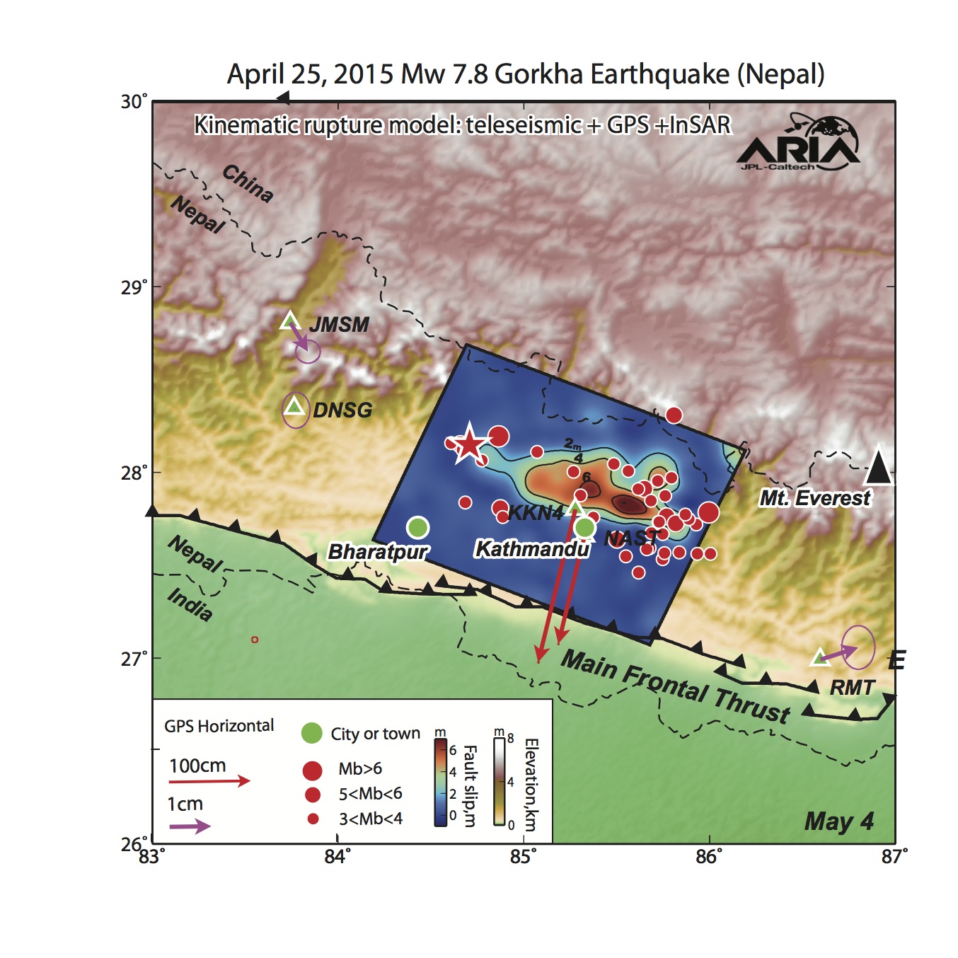
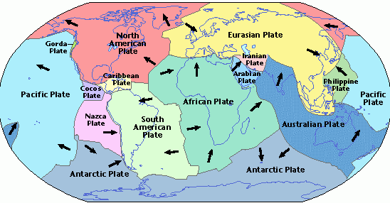
In the first study, the researchers show that the earthquake occurred on the Main Himalayan Thrust (MHT), the main megathrust fault along which northern India is pushing beneath Eurasia at a rate of about two centimeters per year, driving the Himalayas upward. Based on GPS measurements, scientists know that a large portion of this fault is “locked.” Large earthquakes typically release stress on such locked faults–as the lower tectonic plate (here, the Indian plate) pulls the upper plate (here, the Eurasian plate) downward, strain builds in these locked sections until the upper plate breaks free, releasing strain and producing an earthquake. There are areas along the fault in western Nepal that are known to be locked and have not experienced a major earthquake since a big one (larger than magnitude 8.5) in 1505. But the Gorkha earthquake ruptured only a small fraction of the locked zone, so there is still the potential for the locked portion to produce a large earthquake.
“The Gorkha earthquake didn’t do the job of transferring deformation all the way to the front of the Himalaya,” says Avouac. “So the Himalaya could certainly generate larger earthquakes in the future, but we have no idea when.”
The epicenter of the April 25 event was located in the Gorkha District of Nepal, 75 kilometers to the west-northwest of Kathmandu, and propagated eastward at a rate of about 2.8 kilometers per second, causing slip in the north-south direction–a progression that the researchers describe as “unzipping” a section of the locked fault.
“With the geological context in Nepal, this is a place where we expect big earthquakes. We also knew, based on GPS measurements of the way the plates have moved over the last two decades, how ‘stuck’ this particular fault was, so this earthquake was not a surprise,” says Jean Paul Ampuero, assistant professor of seismology at Caltech and coauthor on the Nature Geoscience paper. “But with every earthquake there are always surprises.”
In this case, one of the surprises was that the quake did not rupture all the way to the surface. Records of past earthquakes on the same fault–including a powerful one (possibly as strong as magnitude 8.4) that shook Kathmandu in 1934–indicate that ruptures have previously reached the surface. But Avouac, Ampuero, and their colleagues used satellite Synthetic Aperture Radar data and a technique called back projection that takes advantage of the dense arrays of seismic stations in the United States, Europe, and Australia to track the progression of the earthquake, and found that it was quite contained at depth. The high-frequency waves that were largely produced in the lower section of the rupture occurred at a depth of about 15 kilometers.
“That was good news for Kathmandu,” says Ampuero. “If the earthquake had broken all the way to the surface, it could have been much, much worse.”
The researchers note, however, that the Gorkha earthquake did increase the stress on the adjacent portion of the fault that remains locked, closer to Kathmandu. It is unclear whether this additional stress will eventually trigger another earthquake or if that portion of the fault will “creep,” a process that allows the two plates to move slowly past one another, dissipating stress. The researchers are building computer models and monitoring post-earthquake deformation of the crust to try to determine which scenario is more likely.
Another surprise from the earthquake, one that explains why many of the homes and other buildings in Kathmandu were spared, is described in the Science Express paper. Avouac and his colleagues found that for such a large-magnitude earthquake, high-frequency shaking in Kathmandu was actually relatively mild. And it is high-frequency waves, with short periods of vibration of less than one second, that tend to affect low-story buildings. The Nature Geoscience paper showed that the high-frequency waves that the quake produced came from the deeper edge of the rupture, on the northern end away from Kathmandu.
The GPS records described in the Science Express paper show that within the zone that experienced the greatest amount of slip during the earthquake–a region south of the sources of high-frequency waves and closer to Kathmandu–the onset of slip on the fault was actually very smooth. It took nearly two seconds for the slip rate to reach its maximum value of one meter per second. In general, the more abrupt the onset of slip during an earthquake, the more energetic the radiated high-frequency seismic waves. So the relatively gradual onset of slip in the Gorkha event explains why this patch, which experienced a large amount of slip, did not generate many high-frequency waves.
“It would be good news if the smooth onset of slip, and hence the limited induced shaking, were a systematic property of the Himalayan megathrust fault, or of megathrust faults in general.” says Avouac. “Based on observations from this and other megathrust earthquakes, this is a possibility.”
In contrast to what they saw with high-frequency waves, the researchers found that the earthquake produced an unexpectedly large amount of low-frequency waves with longer periods of about five seconds. This longer-period shaking was responsible for the collapse of taller structures in Kathmandu, such as the Dharahara Tower, a 60-meter-high tower that survived larger earthquakes in 1833 and 1934 but collapsed completely during the Gorkha quake.
To understand this, consider plucking the strings of a guitar. Each string resonates at a certain natural frequency, or pitch, depending on the length, composition, and tension of the string. Likewise, buildings and other structures have a natural pitch or frequency of shaking at which they resonate; in general, the taller the building, the longer the period at which it resonates. If a strong earthquake causes the ground to shake with a frequency that matches a building’s pitch, the shaking will be amplified within the building, and the structure will likely collapse.
Turning to the GPS records from two of Avouac’s stations in the Kathmandu Valley, the researchers found that the effect of the low-frequency waves was amplified by the geological context of the Kathmandu basin. The basin is an ancient lakebed that is now filled with relatively soft sediment. For about 40 seconds after the earthquake, seismic waves from the quake were trapped within the basin and continued to reverberate, ringing like a bell with a frequency of five seconds.
“That’s just the right frequency to damage tall buildings like the Dharahara Tower because it’s close to their natural period,” Avouac explains.
In follow-up work, Domniki Asimaki, professor of mechanical and civil engineering at Caltech, is examining the details of the shaking experienced throughout the basin. On a recent trip to Kathmandu, she documented very little damage to low-story buildings throughout much of the city but identified a pattern of intense shaking experienced at the edges of the basin, on hilltops or in the foothills where sediment meets the mountains. This was largely due to the resonance of seismic waves within the basin.
Asimaki notes that Los Angeles is also built atop sedimentary deposits and is surrounded by hills and mountain ranges that would also be prone to this type of increased shaking intensity during a major earthquake.
“In fact,” she says, “the buildings in downtown Los Angeles are much taller than those in Kathmandu and therefore resonate with a much lower frequency. So if the same shaking had happened in L.A., a lot of the really tall buildings would have been challenged.”
That points to one of the reasons it is important to understand how the land responded to the Gorkha earthquake, Avouac says. “Such studies of the site effects in Nepal provide an important opportunity to validate the codes and methods we use to predict the kind of shaking and damage that would be expected as a result of earthquakes elsewhere, such as in the Los Angeles Basin.”
Video
Between quakes along the Himalaya megathrust, the Indian crust is slowly pulled down under the Himalaya. In some locked zones, the lower plate pulls the upper down, causing the land to subside and stress to build. When stress becomes too great the upper plate breaks free, producing an earthquake. (This animation is not specific to the Gorkha quake, which did not rupture to the surface and propagated parallel to the mountain strike.)
Credit: Jean-Philippe Avouac, Caltech Tectonics Observatory; Tim Pyle, Caltech IPAC
This animation depicts the “unzipping” of a section of the Main Himalayan Thrust during the April 25 earthquake in Gorkha, Nepal. The color-coded circles indicate the sliding velocity at various points along the fault as the rupture propagates eastward. The more irregular, colorful shapes show the sources of high-frequency seismic waves.
Credit: Diego Melgar and Lingsen Meng/Science
References:
Jean-Paul Ampuero et al. Lower edge of locked Main Himalayan Thrust unzipped by the 2015 Gorkha earthquake. Nature Geoscience, August 2015 DOI: 10.1038/ngeo2518
N. Maharjan et al. Slip pulse and resonance of Kathmandu basin during the 2015 Mw 7.8 Gorkha earthquake, Nepal imaged with geodesy. Science Express, August 2015 DOI: 10.1126/science.aac6383
As a devastating earthquake ruptured Nepal on April 25, 2015, nearby GPS networks continuously recorded measurements at very close distances. In a new study, these data provide the scientific community with unique insights into megathrust earthquakes, which occur when two tectonic plates converge and one plate is forced underneath the other, and may help hazard assessment teams improve earthquake hazard models.
To better understand the sudden and intense changes megathrust earthquakes entail, John Galetzka et al. analyzed data from GPS stations located directly above the Main Himalayan Thrust (MHT) thrust fault (the unzipping of which contributed to the Nepal quake), as well as radar measurements that monitored surface displacements. The data from the 2015 earthquake event clearly indicate a pulse-like rupture that occurred over a mere six seconds, just a fraction of the total 70 second-duration of the earthquake.
Measurements reveal a slip pulse 20 kilometers (12.4 miles) wide, with an extremely fast rupture velocity of approximately 3.2km/s (2 miles/second). The smooth onset of the slip pulse limited shaking at frequencies likely to damage regular dwellings, but excited a basin-wide resonance responsible for the collapse of tall structures.
Reference:
“Slip pulse and resonance of Kathmandu basin during the 2015 Mw 7.8 Gorkha earthquake, Nepal imaged with geodesy,” by J. Galetzka; J.F. Genrich; S. Owen; J.-P. Avouac at California Institute of Technology in Pasadena, CA; D. Melgar at University of California, Berkeley in Berkeley, CA; J. Geng; E.O. Lindsey; X. Xu; Y. Bock at University of California, San Diego in La Jolla, CA; S. Owen; A. Moore at Jet Propulsion Laboratory in Pasadena, CA; J.-P. Avouac at University of Cambridge in Cambridge, UK; L.B. Adhikari; P. Shrestha; B. Koirala; U. Gautam; M. Bhatterai; R. Gupta; T. Kandel; C. Timsina; S.N. Sapkota; S. Rajaure; N. Maharjan. DOI: 10.1126/science.aac6383
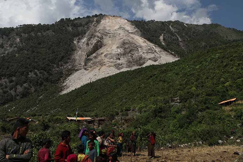
Villagers in Kerauja, Nepal standing below a large rock slide that resulted in one fatality
A new report from the U.S. Geological Survey provides critical landslide-hazard expertise to Nepalese agencies and villages affected by the April 25, magnitude 7.8 earthquake that shook much of central Nepal. The earthquake and its aftershocks triggered thousands of landslides in the steep topography of Nepal, and caused nearly 8,900 fatalities. Hundreds of those deaths were due to landslides, which also blocked vital road and trail lifeline routes to affected villages.
Landslides caused by the earthquakes continue to pose both immediate and long-term hazards to villages and infrastructure within the affected region. Several landslides blocked rivers, creating temporary dams, which were a major concern for villages located downstream. The report provides a rapid assessment of landslide hazards for use by Nepalese agencies during this current monsoon season.
With support from the U.S. Agency for International Development’s Office of U.S. Foreign Disaster Assistance, and in collaboration with earthquake-hazard organizations from both the United States and Nepal, the USGS responded to this landslide crisis by providing expertise to Nepalese agencies and affected villages. In addition to collaborating with an international group of remote-sensing scientists to document the extent and spatial distribution of landsliding in the first few weeks following the earthquake, the USGS conducted in-country landslide hazard assessments for 10 days in May and June. Much of the information obtained by the USGS in Nepal was conveyed directly to affected villages and government agencies as opportunities arose. Upon return to the United States, data organization, interpretation and synthesis immediately began in order to publish a final report.
This new report provides a detailed account of the assessments performed in May and June, with a particular focus on valley-blocking landslides because they have the potential to pose considerable hazard to many villages in Nepal. The results include an overview of the extent of landsliding, a presentation of 74 valley-blocking landslides identified during the work, and a description of helicopter-based video resources that provide over 11 hours of high resolution footage of approximately 1,000 km (621 miles) of river valleys and surrounding areas affected by the earthquakes. A description of site-specific landslide-hazard assessments conducted while in Nepal and detailed descriptions of five noteworthy case studies are also included. The report ends with an assessment of the expectation for additional landslide hazards in the summer monsoon season following the earthquakes.
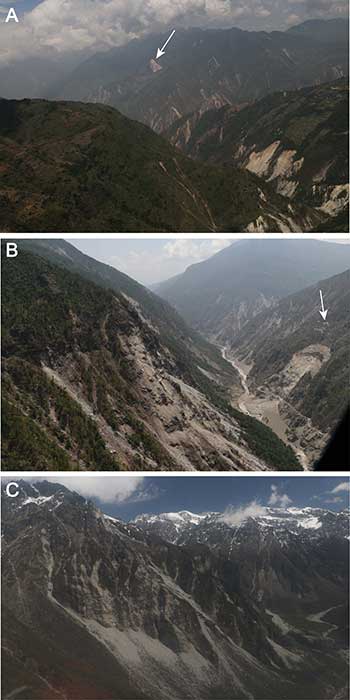
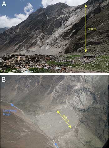
Aerial photographs showing landslides triggered by the April and May 2015 Gorkha earthquake sequence in central Nepal. A, Widespread ridgetop landsliding in Gorkha district. The Kerauja rock slide (cover image of report) is wide scar on ridge visible in photograph background (arrow). B, Partially breached Gogane landslide dam in Rasuwa district of Nepal. Top of scarp below village (arrow) is approximately 400 m above river level. C, Rock falls in the Urkin Kangari Valley, Sindhupalchok district. Image shows approximately 1,200 m relief between top of foreground cliffs and valley floor.Photographs showing the Langtang, Nepal debris avalanche, which destroyed the entire village of Langtang. An estimated 200 people were killed in this single event. A, Oblique northwest view of deposit with cliff in which the debris became airborne. Homes in foreground were pushed over by the ensuing airblast. B, Aerial view of debris avalanche deposit showing location of the Langtang River tunnel through ice and debris.
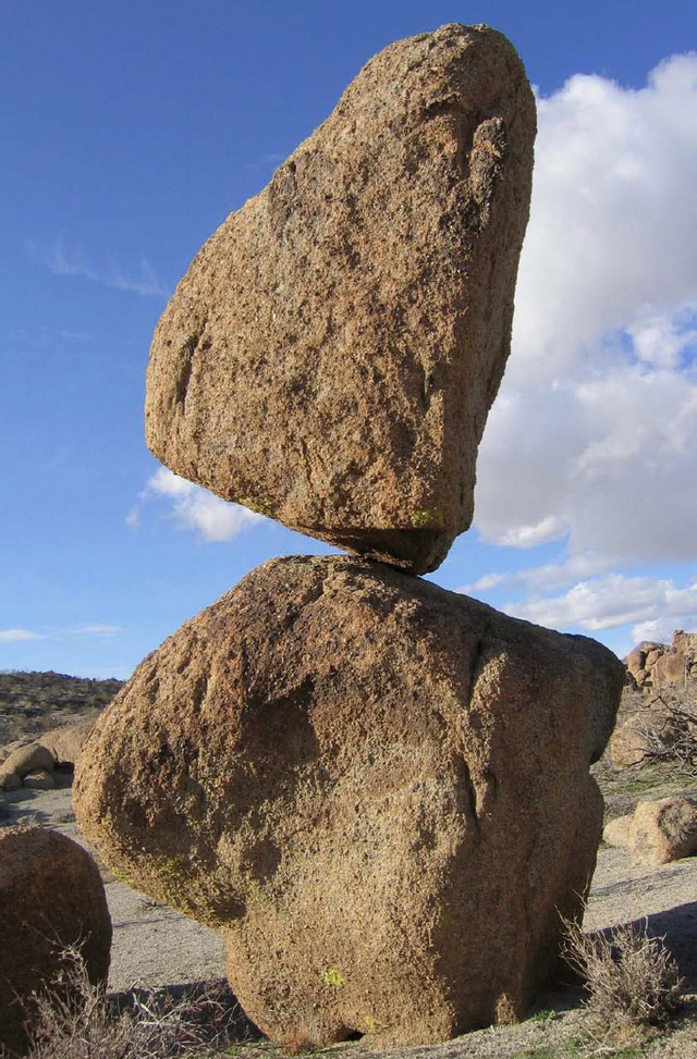
A precariously balanced rock near Searchlight, Nev. Fragile features such as this are easily toppled by shaking from strong earthquakes. Similar formations near California’s San Andreas Fault provide critical insights into the shaking and rupture patterns of past earthquakes. Credit: Nick Hinze / Nevada Bureau of Mines & Geology
Stacked in gravity-defying arrangements in the western San Bernardino Mountains, granite boulders that should have been toppled long ago by earthquakes are maintaining a stubborn if precarious balance. In puzzling out why these rocks still stand, researchers have uncovered connections between Southern California’s San Jacinto and San Andreas faults that could change how the region plans for future earthquakes.
In their study published online August 5 in Seismological Research Letters (SRL), Lisa Grant Ludwig of University of California, Irvine and colleagues write that the precariously balanced rocks (PBRs) have survived as a result of interactions between the faults that have weakened earthquake ground shaking near the rocks.
One such interaction, the researchers say, might be a rupture that began on the San Andreas Fault but then jumped over to the San Jacinto Fault, near Cajon Pass. “These faults influence each other, and it looks like sometimes they have probably ruptured together in the past,” said Grant Ludwig. “We can’t say so for sure, but that’s what our data point toward, and it’s an important possibility that we should think about in doing our earthquake planning.”
Cajon Pass is the site of “some very important, lifeline infrastructure like I-15, and we should be considering the possibility that there might be broader disruptions in that area,” Grant Ludwig added.
Most of the seismic hazard maps that engineers and others use to guide the design of buildings, aqueducts and other important infrastructure often only account for the ground shaking and other impacts produced by ruptures along one fault, she noted.
“This paper suggests that we might consider the impact of a rupture that involves both the San Jacinto and San Andreas Faults, which has the potential to affect more people than just the San Andreas or just the San Jacinto,” Grant Ludwig said.
The precariously balanced rocks (PBRs) analyzed in the SRL study are part of a massive PBR dataset developed by co-author James Brune and his research group at the University of Nevada, Reno. Grant Ludwig, Brune, and their colleagues examined 36 PBRs near Silverwood Lake and Grass Valley that lay only seven to 10 kilometers away from the San Andreas or San Jacinto Faults. The PBRs are at least 10,000 years old, and should have experienced ground shaking from 50 to 100 large, surface-rupturing earthquakes over that time.
Scientists measure the fragility of these rocks by studying their geometry and doing field tests like tilt analyses, where they put a pulley on a PBR and measure the force required to “tilt it to the point where if you let it go, it will fall under the influence of gravity,” Grant Ludwig explained.
The researchers report this force as a measure of acceleration. Just a person in the passenger seat of a car tilts back when the driver steps on the gas pedal, the PBRs tilt in response the ground accelerating beneath them as the result of an earthquake. Ludwig also compared the phenomenon to pulling a small rug out from under a tower of Lego blocks. The higher the acceleration of the pulled rug, the more likely it is that it will topple the tower.
Ludwig and colleagues compared PBR fragilities with the expected acceleration of the ground in three earthquake scenarios created by the U.S. Geological Survey’s “ShakeMap” program: a magnitude 7.8 rupture of the southern San Andreas Fault, a magnitude 7.4 San Andreas quake near San Bernardino, and the 1857 magnitude 7.9 Fort Tejon earthquake.
These earthquake scenarios, along with National Seismic Hazard Maps for the area, predicted that these 36 PBRs would have toppled a long time ago. “It was a real scientific puzzle, a real head-scratcher,” said Grant Ludwig. “How can you have these rocks right next to the San Andreas Fault? It’s an interesting scientific question, but it also has practical implications, because we want our seismic hazard maps to be as good as possible.”
After a decade’s work investigating many possible answers to the puzzle, the researchers concluded that only interactions between the San Jacinto and San Andreas Faults could have produced the kind of rupture pattern that would preserve the area’s precariously balanced rocks.
Recognizing this interaction between the two major faults could change earthquake planning scenarios for the area, Ludwig concluded.
“The San Jacinto fault has been very seismically active. It has produced a lot of earthquakes during the historic period. And the Southern San Andreas fault has not, it has been pretty quiet since 1857,” she said. “This brings up the question of whether we might have an earthquake on the San Jacinto that triggers one on the Southern San Andreas, or vice versa.”
Reference:
The study, “Reconciling precariously balanced rocks (PBRs) with large earthquakes on the San Andreas fault system,” will be published online August 5 and in the September/October print edition of SRL. The Seismological Society of America publishes the journal SRL.
New research by scientists at New Zealand’s University of Otago and GNS Science is helping to solve the puzzle of how bacteria are able to live in nutrient-starved environments. It is well-established that the majority of bacteria in soil ecosystems live in dormant states due to nutrient deprivation, but the metabolic strategies that enable their survival have not yet been shown.
The researchers took an extreme approach to resolving this enigma.
They studied a strain of acidobacteria named Pyrinomonas methylaliphatogenes that was cultivated from heated and acidic geothermal soils in New Zealand’s Taup? Volcanic Zone. Remarkably, the bacterium was living in this inhospitable ecosystem despite its soil lacking the nutrients the microbe usually relied on.
Following in-depth studies on the genetic and biochemical capabilities of the organism, the authors uncovered that the bacterium actually took a highly minimalistic approach to survival. When its preferred carbohydrate nutrient sources are exhausted, it is able to scavenge trace amounts of the fuel hydrogen from the air. To survive, the organism simply requires atmospheric hydrogen and oxygen. It is ‘living on thin air’, so to speak.
The findings appear in the journal Proceedings of the National Academy of Sciences (PNAS). The paper co-authors include the Department of Microbiology and Immunology’s Professor Greg Cook, his past PhD student Dr Chris Greening (now CSIRO) and GNS Science researchers Dr Matthew Stott and Dr Carlo Carere.
By focusing on a slow-growing isolate rather than a typical fast-growing lab strain, the team were able to get rich insight into the survival strategies of the ‘dormant microbial majority’. Professor Cook says this is the first time that acidobacteria — the second most dominant bacteria in global soils — have been found to be able to consume hydrogen gas as an energy source. “Even though there are only low concentrations of the gas in the air, it still provides them with a constant and unlimited resource for survival,” he says.
This publication is the latest in a trilogy of PNAS papers authored by Professor Cook and Dr Greening. Their other recent work showed that soil actinobacteria, another dominant phylum, demonstrate a similar metabolic flexibility in switching to scavenging hydrogen when starved of other nutrients.
In their latest paper, the researchers conclude by proposing that scavenging of trace gases such as hydrogen is an under-recognised general mechanism for bacterial survival and is likely to provide the energy to sustain a significant proportion of the bacterial communities in soils.
Reference:
Chris Greening, Carlo R. Carere, Rowena Rushton-Green, Liam K. Harold, Kiel Hards, Matthew C. Taylor, Sergio E. Morales, Matthew B. Stott, Gregory M. Cook. Persistence of the dominant soil phylumAcidobacteriaby trace gas scavenging. Proceedings of the National Academy of Sciences, 2015; 201508385 DOI: 10.1073/pnas.1508385112
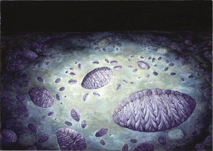
Artist’s reconstruction of the Fractofusus community on the H14 surface at Bonavista Peninsula showing the clusters that arise from stolon-like reproduction. The large individuals represent the primary colonizers of the site. Their offspring cluster around them, and are themselves surrounded by their own offspring – the third generation on the bed. The stolon-like protrusions are faintly visible and weave in and out of the microbial mat which covers the seafloor. Lighting is artificial and as though from a submersible ROV. Credit: C. G. Kenchington
Researchers led by the University of Cambridge have found the earliest example of reproduction in a complex organism. Their new study has found that some organisms known as rangeomorphs, which lived 565 million years ago, reproduced by taking a joint approach: they first sent out an ‘advance party’ to settle in a new area, followed by rapid colonisation of the new neighbourhood. The results, reported today in the journal Nature, could aid in revealing the origins of our modern marine environment.
Using statistical techniques to assess the distribution of populations of a type of rangeomorph called Fractofusus, the researchers observed that larger ‘grandparent’ rangeomorphs were randomly distributed in their environment, and were surrounded by distinct patterns of smaller ‘parents’ and ‘children’. These patterns strongly resemble the biological clustering observed in modern plants, and suggest a dual mode of reproduction: the ‘grandparents’ being the product of ejected waterborne propagules, while the ‘parents’ and ‘children’ grew from ‘runners’ sent out by the older generation, like strawberry plants.
Rangeomorphs were some of the earliest complex organisms on Earth, and have been considered to be some of the first animals — although it’s difficult for scientists to be entirely sure. They thrived in the oceans during the late Ediacaran period, between 580 and 541 million years ago, and could reach up to two metres in length, although most were around ten centimetres. Looking like trees or ferns, they did not appear to have mouths, organs, or means of moving, and probably absorbed nutrients from the water around them.
Like many of the life forms during the Ediacaran, rangeomorphs mysteriously disappeared at the start of the Cambrian period, which began about 540 million years ago, so it has been difficult to link rangeomorphs to any modern organisms, or to figure out how they lived, what they ate and how they reproduced.
“Rangeomorphs don’t look like anything else in the fossil record, which is why they’re such a mystery,” said Dr Emily Mitchell, a postdoctoral researcher in Cambridge’s Department of Earth Sciences, and the paper’s lead author. “But we’ve developed a whole new way of looking at them, which has helped us understand them a lot better — most interestingly, how they reproduced.”
Mitchell and her colleagues used high-resolution GPS, spatial statistics and modelling to examine fossils of Fractofusus, in order to determine how they reproduced. The fossils are from south-eastern Newfoundland in Canada, which is one of the world’s richest sources of fossils from the Ediacaran period. Since rangeomorphs were immobile, it is possible to find entire ecosystems preserved exactly where they lived, making them extremely suitable for study via spatial techniques.
The ‘generational’ clustering patterns the researchers observed fit closely to a model known as a nested double Thomas cluster model, of the type seen in modern plants. These patterns suggest rapid, asexual reproduction through the use of stolons or runners. At the same time, the random distribution of larger ‘grandparent’ Fractofusus specimens suggests that they were the result of waterborne propagules, which could have been either sexual or asexual in nature.
“Reproduction in this way made rangeomorphs highly successful, since they could both colonise new areas and rapidly spread once they got there,” said Mitchell. “The capacity of these organisms to switch between two distinct modes of reproduction shows just how sophisticated their underlying biology was, which is remarkable at a point in time when most other forms of life were incredibly simple.”
The use of this type of spatial analysis to reconstruct Ediacaran organism biology is only in its infancy, and the researchers intend to extend their approach to further understand how these strange organisms interacted with each other and their environment.
The research was funded by the Natural Environment Research Council.
Reference:
Emily G. Mitchell, Charlotte G. Kenchington, Alexander G. Liu, Jack J. Matthews, Nicholas J. Butterfield. Reconstructing the reproductive mode of an Ediacaran macro-organism. Nature, 2015; DOI: 10.1038/nature14646
Note: The above post is reprinted from materials provided by University of Cambridge. The original story is licensed under a Creative Commons Licence.
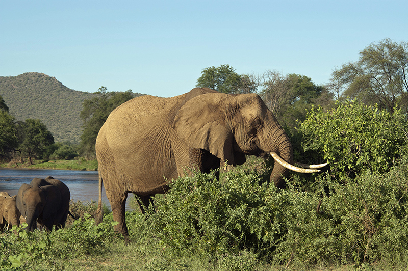
An African elephant browses on shrubs at Kenya’s Samburu National Reserve. A new University of Utah study found that elephants, like many African animals, tried grazing on grass during the past 4 million years, but eventually switched to browsing on trees and shrubs like the African elephant or went extinct, like the Asian elephant did in Africa, even though it survives in Asia. Photo Credit: Mahala Kephart
As grasses grew more common in Africa, most major mammal groups tried grazing on them at times during the past 4 million years, but some of the animals went extinct or switched back to browsing on trees and shrubs, according to a study led by the University of Utah.
“It’s as if in a city, there was a whole new genre of restaurant to try,” says geochemist Thure Cerling, first and senior author of the study published by the journal Proceedings of the National Academy of Sciences. “This is a record of how different mammals responded. And almost all of the mammals did an experiment in eating this new resource: grass.”
The experiment peaked about 2 million years ago, says Cerling, a distinguished professor of geology and geophysics. The only major group that still mostly grazes grass is the bovids: cattle, buffalo, sheep, wildebeest, hartebeest and some antelopes such as oryx and waterbucks.
The study also revealed that the present isn’t necessarily the key to the past in terms of what animals eat. Today, elephants and spiral-horned antelope (elands, kudus and bushbuck) browse on trees and shrubs, but the study showed that 2 million years ago, African elephants grazed on grass and the antelopes had mixed diets with a lot of grass. Asian elephants, which ate grass and were abundant in Africa 2 million years ago, went extinct in Africa but survive in Asia, where they graze but also browse trees and shrubs.
“That the diet of some of these animals is different from that of the present was a surprise, and shows the importance of challenging one’s assumptions when making ecological reconstructions,” says study co-author and geologist Frank Brown, dean of the University of Utah’s College of Mines and Earth Sciences.
Overall, Cerling and colleagues wrote that the assemblages of grazing, browsing and mixed-diet animals during the past 4 million years “are different from any modern ecosystem in East or Central Africa.”
They found the Turkana Basin of Kenya and Ethiopia had a much greater diversity of mixed feeders — they browsed and grazed — from 4.1 million to 2.35 million years ago. From 2.35 million to 1 million years ago, there were many more grazers than there are today. In the past 1 million years, many grass grazers either switched to browsing trees and shrubs or went extinct, leaving mostly bovids as grazers today.
The study was funded by the Fulbright Foundation, the University of Utah, the Geological Society of America, the National Science Foundation, the Packard Foundation and the National Geographic Society.
30 years of research into 4 million years of dietary evolution
In a study spanning 30 years of field work by Cerling into how grasses and the animals that eat them evolved together, he and other scientists analyzed:
Hair keratin, tooth enamel or bone collagen from 1,800 animals of more than 50 modern herbivore species in East and Central Africa. Samples came from museum collections or from animals killed previously in 30 national parks and reserves.
Tooth enamel from more than 900 fossil herbivores that lived 4.1 million to 1 million years ago in the Turkana Basin.
They measured the samples’ ratios of uncommon carbon-13 to common carbon-12. The ratios reveal if the animals browsed primarily on plants that use C3 photosynthesis (trees, shrubs, forbs and herbs), grazed mainly on C4 photosynthesis plants (dry-season or tropical grasses and sedges) or ate a mixed diet.
Low carbon dioxide levels in the atmosphere are believed responsible for a global expansion of tropical grasslands between 10 million and 5 million years ago. C4 photosynthesis used by tropical grasses is more efficient in hot climates, giving them an advantage over trees and shrubs.
“Over the past 10 million years, grasses went from perhaps 1 percent of productivity of the tropical landscape to 50 percent today,” Cerling says. “All the large mammal groups tried experiments in eating grasses, and a lot of those experiments didn’t work in the long run,” he says. “Animals became extinct or they switched to other diets. There was even a grazing giraffe, but that became extinct. There were three major lineages of pigs that were grazers, and only one has survived: the warthog.”
Other grazers that became extinct included a three-toed horse and the Asian elephant, which survives in Asia but went extinct in Africa 1 million years ago.
Grazers that switched to browsing included forest hogs and African elephants.
Browsers in the past that still browse at least 75 percent trees and shrubs today include most giraffes, black rhinos, tiny antelope and forest antelope.
One-toed horses, warthogs, zebras, white rhinos and bovids — cattle, buffalo, goats, wildebeest, hartebeest and antelopes like waterbuck and oryx — stuck with grass.
“The successful grazers appear to be the bovids,” Cerling says, although even some bovids — gazelles and elands — once were mixed grazers-browsers, but today have returned to mostly browsing on trees and shrubs. Impalas, which also are bovids, shifted from mostly grazing in the past to both grazing and browsing today.
Modern herbivores with mixed browsing-grazing diets include hippos and impalas.
Why did the grass craze fade?
Why did some animals keep eating grass while others stopped or went extinct?
“Perhaps they were much more efficient at eating grass and outcompeted some of the other animals,” Cerling says. For example, perhaps African elephants switched to browsing when they could no longer grab grass cut too short by grazers.
“It looks like there is as much grass available now as anytime in the past,” Cerling says. “It could be that the quality of grass varies enormously between the dry season and the wet season.”
He also notes that during the past 1 million years, “we have been going through strong cycles with and without glaciers, and much bigger changes in atmospheric carbon dioxide.” Grasses using C4 photosynthesis not only have an advantage in hot weather, but also during glacial periods when carbon dioxide levels were low.
But there are no fossils of grasses for the past 10 million years, which makes it difficult to unveil the evolution of grasses, and whether they changed in digestibility, palatability, toxin levels and nutrient content, Cerling says.
In a 2013 study, Cerling found that early human relatives who turned to grazing, such as Paranthropus boisei, went extinct. Modern humans eat more grass than ever before — but not by grazing. Instead, we eat the meat of animals fed grass and C4 grains, as well as cultivated C4 plants such as corn and sorghum.
Reference:
Thure E. Cerling, Samuel A. Andanje, Scott A. Blumenthal, Francis H. Brown, Kendra L. Chritz, John M. Harris, John A. Hart, Francis M. Kirera, Prince Kaleme, Louise N. Leakey, Meave G. Leakey, Naomi E. Levin, Fredrick Kyalo Manthi, Benjamin H. Passey, and Kevin T. Uno. Dietary changes of large herbivores in the Turkana Basin, Kenya from 4 to 1 Ma. PNAS, July 2015 DOI: 10.1073/pnas.1513075112
Imagine a world without liquid water—just solid ice in all directions. It would certainly not be a place that most life forms would like to live.
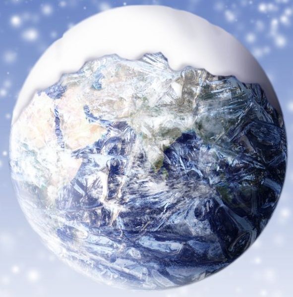
And yet our planet has gone through several frozen periods, in which a runaway climate effect led to global, or near global, ice cover. The last of these so-called “Snowball Earth” glaciations ended around 635 million years ago when complex life was just starting to develop. It’s still uncertain if ice blanketed the entire planet, or if some mechanism was able to halt the runaway.
“Studying Snowball Earth glaciations can tell us just how bad it can get, in which case life as we know it would probably not survive,” says geologist Linda Sohl of Columbia University.
Sohl and her colleagues are taking global climate models—the ones most people use to predict where our planet is heading in the future—and modifying them to study where our planet has been in the past.
In their simulations of the Cryogenian period (850-635 million years ago), the group has found that the Earth’s global mean temperature could have fallen 12 degrees Celsius below freezing, and yet the world would not completely freeze over. The models predict that half of the oceans remain ice-free even under these extreme conditions. The implication is that Earth resisted snowballing into a solid ice ball at this crucial point in Earth’s history.
The team has received a grant from the Exobiology & Evolutionary Biology element of the NASA Astrobiology Program to explore other Snowball Earth scenarios. The goal is to identify which factors, such as the arrangement of continents and ocean circulation, play a role in driving glaciation or halting it.
The results could influence discussions on the limits of habitability around other stars. Water-bearing planets like Earth may carry some natural defense mechanism against global freezing, and this might mean liquid water is more common in the Universe than astrobiologists have traditionally assumed.
Hard or slushy
Scientists contend that at least two Snowball Earth glaciations occurred during the Cryogenian period, roughly 640 and 710 million years ago. Each lasted about 10 million years or so.
The main evidence of the severity of these events comes from geological evidence of glaciers near the equator. If ice on land made it down to the low latitudes, as the argument goes, then it must have gone everywhere.
This “all in” climate response is due to the high reflectivity, or albedo, of ice. Ice reflects 55 to 80 percent of incoming sunlight, sending that energy back into space before it can warm the planet. By comparison, ocean water reflects just 12 percent, and land areas reflect between 10 and 40 percent, so more of the sun’s heat is absorbed by these surface conditions. An additional factor in cooling the planet is that the Sun was 6 percent fainter during the Cryogenian period than it is now.
Early models showed that once ice reached tropical latitudes, a positive feedback loop would take hold, in which ice cover would lead to lower temperatures, which would add more ice cover, which would lower temperatures even more. This runaway effect would presumably continue until the entire planet froze over, with even the oceans covered with as much as a kilometer-thick layer of ice.
This so-called “hard snowball” would lock the planet into an eternal winter, à la the Disney hit, “Frozen.” The difference is that no magical spells exist to release a Snowball Earth from such a deep freeze.
Indeed, scientists have had a hard time explaining how a hard snowball could ever thaw. One proposal is that volcanic activity releases greenhouse gases that eventually warm the planet back up. The amount of carbon dioxide (CO2) needed might be several hundred times higher than what our atmosphere contains now. However, there is no geologic evidence to support that much CO2 in the Cryogenian atmosphere, Sohl says.
Another problem for the hard snowball theory is the lack of a massive extinction event in the Cryogenian fossil record. One would expect a major hit to the ocean ecosystem when it presumably got cut off from the Sun by a thick layer of ice, but only relatively small extinctions have been found.
A further complication is evidence of an ongoing water cycle during the Cryogenian. Such precipitation runs counter to the dry atmosphere that would likely develop if the oceans were all capped with ice.
“The suggestion that the Earth was once entirely covered by ice—the continents by thick ice sheets and the oceans by thick sea ice—remains somewhat contentious,” says physicist Richard Peltier of the University of Toronto.
In response to these concerns, an alternative theory has developed that goes by the name “slushball.” In this case, the Earth becomes largely covered with ice, but open water remains near the equator. Sohl says that many of her geologist colleagues lean toward the slushball scenario, as it seems to better match observations.
That is not to say that a hard snowball never happened. Extensive glaciation took place around 2.2 billion years ago, in the Paleoproterozoic era, and it seems plausible that global ice cover occurred then, Sohl says. Compared to the Cryogenian, the Paleoproterozoic sun was even fainter (down 16 percent in brightness from now). The timing of the glaciation also seems to coincide with the evolution of photosynthetic life, which would have drastically reduced greenhouse gases through the release of oxygen.
Tuning for the past
To give a better understanding of the contentious Cryogenian period, Sohl’s team has been developing climate models that recreate the conditions on Earth nearly a billion years ago.
They start with the NASA/GISS Earth System Model (ModelE2-R), which has been used to make the most recent climate assessments by the Intergovernmental Panel on Climate Change (IPCC). But they turn the clock back on the simulation, altering the parameters to what they were in the past. For example, the Sun’s brightness is dimmed by 6 percent and the continents are arranged into a single supercontinent near equator.
“You need this flexibility when studying past climate conditions,” Sohl says. “We are probably using one of the most sophisticated models available for our paleoclimate runs.”
Some previous attempts at simulating Earth’s history have focused on explicitly trying to produce a hard snowball, but Sohl and her colleagues have preferred to let the climate model suggest what the outcome of their runs should be. They have found that ocean currents, like the present-day Gulf Stream, have a large impact on how and where heat from the Sun ends up distributed across the Earth’s surface.
“For us, the ocean circulation seems to help in preventing a full freeze-over,” Sohl says.
The team’s early results show that the ocean retains areas of open water in the tropics, even when glaciers cover much of the land mass. The implication seems to be that the slushball picture is more likely than the hard snowball, at least as far as the Cryogenian period is concerned.
Sohl and her colleagues are now exploring other aspects that could play a role in past climates. For example, the day was shorter during the Cryogenian (21.9 hours instead of 24), and that likely affected the atmospheric dynamics.
Peltier, who is not involved in this work, believes one of the most outstanding issues remaining in Snowball Earth studies is the effect of the topography (i.e., altitude variations). Higher topography could enable glaciation even when other factors work against it, he says.
Other ice worlds
These are not the first climate simulations to show that freezing a planet is not so easy, but “the message hasn’t really gotten to the astrobiologists” Sohl says. The astrobiology community tends to think of the hard snowball as the cold edge of habitability. They are often unaware how “slushy” that edge can be.
The traditional definition of planet habitability is the presence of liquid water. And for convenience, scientists often assume that the state of water is determined by the distance a planet is from its star. In which case, the “habitable zone” is the region around a star where liquid water should exist. A planet outside this habitable zone should be in permanent snowball territory.
But those who study climate know that an awful lot of factors go into freezing besides just the star-to-planet distance. Through her current project, Sohl hopes to elucidate some of these factors.
“In the end, I think we’ll come to realize that the habitable zone is broader than we originally thought,” she says.
Note: The above post is reprinted from materials provided by Astrobio.net. This story is republished courtesy of NASA’s Astrobiology Magazine.
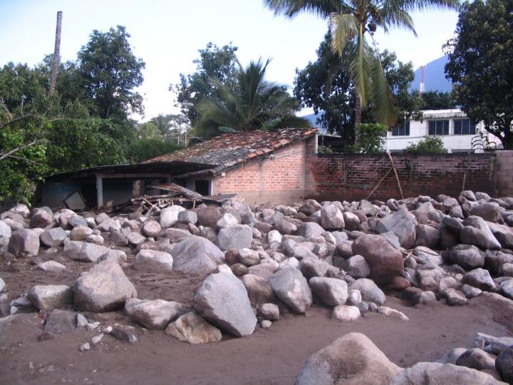
Landslides on the slopes of volcanoes threaten communities like this one in El Salvador. Credit: Michigan Tech, Jose Fredy Cruz
In October 2011, heavy rainfall poured down the sides of El Salvador’s San Vicente Volcano, nearly four feet of water in 12 days. Coffee plantation employees, working high up on the volcano’s slope began noticing surface cracks forming on steep slopes and in coffee plantations. Cracks herald landslides—places where the wet, heavy upper layers, saturated with water, slide over the less-permeable rocky layers underneath. The workers radioed downslope, keeping close tabs on the rainfall gauge network.
Luke Bowman was also there, helping direct radio calls and conducting fieldwork. Bowman, who recently defended his doctoral research in geology at Michigan Technological University, studies geohazards on San Vicente. The Journal of Applied Volcanology recently published some of his research, co-authored by Kari Henquinet, director of the Michigan Tech Peace Corps Master’s International Program and a senior lecturer in the Department of Social Sciences. Their work combines traditional hazard assessments with social science techniques to develop a more in-depth understanding of the risks present at San Vicente Volcano in El Salvador.
San Vicente
Fire, brimstone and destruction dominate the portrayal of volcanoes around the world. But in reality, a number of people live on their slopes. For these communities, eruptions are only one of the risks—other geohazards like landslides (lahars) and flooding pose more frequent threats.
The 2011 rainstorms in El Salvador are a case in point as well as a testament to the importance of expanding geohazards studies to include the people they affect.
“In 2009, as heavy rains fell on San Vicente volcano, most people were waiting for civil protection to issue a warning—and that warning never came,” Bowman says, adding that a landslide crashed down the volcano that year, and many communities within the five municipalities that encompass the northern flank of the volcano were affected, with homes and properties destroyed, infrastructure damaged and lives lost.
“Now, after significant changes in monitoring and reporting hazards, local residents are the ones who gather the rainfall rate data, who measure the cracks and who report it around the community to each other,” Bowman says. “I think it gives people some say in the decisions being made.”
Empowering communities is part of what Bowman hopes to do with his research, but he says it goes beyond just including local citizens in data gathering.
“No matter how good the science is, or how well we can predict where a hazard could occur, there’s still a human component we shouldn’t ignore,” Bowman says, adding that local communities often have a stronger working knowledge of a place than outside researchers. He says researchers can be of greater help when they have a clearer understanding of the broader social and cultural context of geohazards.
Social Geology
Merging geoscience and social science research is called “social geology”—a term coined by Bill Rose, professor-emeritus in the Department of Geological and Mining Engineering and Sciences at Michigan Tech. The interdisciplinary work is a key part of the research conducted by both Rose and John Gierke, the chair of the Department of Geological and Mining Engineering and Sciences.
“Most people think of geologists as just going out and identifying rocks,” Gierke says, explaining that geoscience is much broader and that researchers try to understand how the earth works. “And there’s a growing interest in having a stronger connection between physical science work and the impacts on communities.”
Gierke, who was Bowman’s PhD co-advisor with Rose, says bridging the social and physical worlds is a focus of the studies in Michigan Tech’s Peace Corps Master’s International Program. Bowman, who served in the Peace Corps in Honduras before his graduate studies, is a model for other geoscience and Peace Corps students looking to broaden their physical science research.
Ethnography
Incorporating social science techniques—like ethnographic interviews and participatory observations of community meetings—is no easy feat for physical scientists, who have not been trained to think that way. Collaboration is important, and Henquinet worked with Bowman on his volcanology research to round out his social science data gathering methodology.
“The ethnographic approach is immersion,” Henquinet says, explaining researchers have to learn in the field and adjust their work accordingly. “It’s an approach that’s exploratory, grounded in reality and the context that people live in, so you’re not isolating or manipulating an experiment in a lab.”
For the San Vicente studies, Bowman analyzed quantitative physical data—everything from rainfall to slope stability calculations—along with qualitative social data from one-on-one interviews, community gatherings and key documents. As a result, he and Henquinet were able to delve deeper into the socio-economic limits that forced people to live in active landslide zones. That also enabled them to suggest more realistic evacuation plans and emergency protocols because the local communities were invested participants in the work, plus social vulnerability was accounted for in addition to geophysical vulnerability.
“At the end of the day, there are a lot of political issues that have to be considered in understanding vulnerability and inequalities,” Henquinet says, explaining that the San Vicente research is a small step across a big gap in socio-economic conditions. “Countries like El Salvador are rich with people with ideas—if we want to give these ideas a chance in combating poverty, then give people who live there more voice to work in partnerships.”
Although small in the world’s grand scheme of politics and volcanoes, San Vicente is an example of how people can make a difference. Henquinet and Bowman both say they hope their research has contributed to those changes and that more physical scientists are inspired to collaborate with social scientists too.
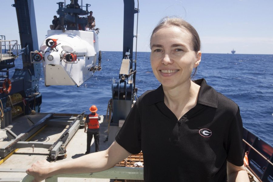
Samantha Joye is a professor of marine sciences in the University of Georgia Franklin College of Arts and Sciences. Credit: Courtesy of Todd Dickey/University of Georgia
The study, published in Nature Communications by Samantha Joye and colleagues, describes how high rates of anaerobic methane oxidation, a process once considered insignificant in these environments, substantially reduce atmospheric emissions of methane from freshwater wetlands.
While anaerobic methane oxidation in freshwaters has been gathering scientific attention, the environmental relevance of this process was unknown.
“This paper reports a previously unrecognized sink for methane in freshwater sediments, soils and peats: microbially mediated anaerobic oxidation of methane,” said Joye, UGA Athletic Association Professor of Arts and Sciences and a professor of marine sciences. “The fundamental importance of this process in freshwater wetlands across broad biogeographic provinces underscores the critical role that anaerobic oxidation of methane plays on Earth, even in freshwater habitats.”
Joye noted that absent this process, methane emissions from freshwater wetlands could be 30 to 50 percent greater.
“This study furthers the understanding of the global methane budget and may have ramifications for the development of future greenhouse gas models,” said study co-author Katherine Segarra, an oceanographer at the U.S. Department of the Interior’s Bureau of Ocean Energy Management.
The research team investigated the anaerobic oxidation process at three freshwater wetlands in three biogeographical regions: the freshwater peat soils of the Florida Everglades; a coastal organic-rich wetland in Acadia National Park, Maine; and a tidal freshwater wetland in coastal Georgia. All three sites were sampled over multiple seasons.
The anaerobic oxidation of methane was coupled, to some extent, to sulfate reduction. Rising sea levels, for example, would result in increased sulfate, which could fuel greater rates of anaerobic oxidation. Similarly, with saltwater intrusion into coastal freshwater wetlands, increasing sulfate inhibits the microbial methane formation, or methanogenesis.
So while freshwater wetlands are known to be significant methane sources to the atmosphere, their low sulfate concentrations previously led most to conclude that anaerobic oxidation of methane was not important in these regions. The new study shows that if not for the anaerobic methane oxidation process, freshwater environments would account for an even greater portion of the global methane budget.
“The process of anaerobic oxidation of methane in freshwater wetlands appears distinct in some regards to what we know about this process in marine sediments,” Joye said. “There could be unique biochemistry, because the isotopic signature of the biomass of microorganisms oxidizing methane in freshwater wetlands is different from their marine counterparts. This could mean that the mechanisms by which they assimilate carbon into their biomass is distinct and/or that different microorganisms carry out anaerobic oxidation of methane in freshwater habitats.”
Reference:
K. E. A. Segarra, F. Schubotz, V. Samarkin, M. Y. Yoshinaga, K-U Hinrichs, S. B. Joye. High rates of anaerobic methane oxidation in freshwater wetlands reduce potential atmospheric methane emissions. Nature Communications, 2015; 6: 7477 DOI: 10.1038/ncomms8477
Note: The above post is reprinted from materials provided by University of Georgia. The original item was written by Alan Flurry.
Though they occupy a small fraction of Earth’s surface, freshwater wetlands are the largest natural source of methane going into the atmosphere. New research from the University of Georgia identifies an unexpected process that acts as a key gatekeeper regulating methane emissions from these freshwater environments.
North America may have once been attached to Australia, according to research just published in Lithosphere and spearheaded by U.S. Geological Survey geologist James Jones and his colleagues at Bucknell University and Colorado School of Mines.
Approximately every 300 million years, the Earth completes a supercontinent cycle wherein continents drift toward one another and collide, remain attached for millions of years, and eventually rift back apart. Geologic processes such as subduction and rifting aid in the formation and eventual break-up of supercontinents, and these same processes also help form valuable mineral resource deposits. Determining the geometry and history of ancient supercontinents is an important part of reconstructing the geologic evolution of Earth, and it can also lead to a better understanding of past and present mineral distributions.
North America is a key component in reconstructions of many former supercontinents, and there are strong geological associations between the western United States and Australia, which is one of the world’s leading mineral producers.
In this study, Jones and others synthesized mineral age data from ancient sedimentary rocks in the Trampas and Yankee Joe basins of Arizona and New Mexico. They found that the ages of many zircon crystals—mineral grains that were eroded from other rocks and embedded in the sedimentary deposits—were approximately 1.6 to 1.5 billion years old, an age range that does not match any known geologic age provinces in the entire western United States.
This surprising result actually mirrors previous studies of the Belt-Purcell basin (located in Montana, Idaho and parts of British Columbia, Canada) and a recently recognized basin in western Yukon, Canada, in which many zircon ages between 1.6 and 1.5 billion years old are common despite the absence of matching potential source rocks of this age.
However, the distinctive zircon ages in all three study locations do match the well known ages of districts in Australia and, to a slightly lesser known extent, Antarctica.
This publication marks the first time a complete detrital mineral age dataset has been compiled to compare the Belt basin deposits to strata of similar age in the southwestern United States. “Though the basins eventually evolved along very different trajectories, they have a shared history when they were first formed,” said Jones. “That history gives us clues as to what continents bordered western North America 1.5 billion years ago.”
The tectonic model presented in this paper suggests that the North American sedimentary basins were linked to sediment sources in Australia and Antarctica until the break up of the supercontinent Columbia. The dispersed components of Columbia ultimately reformed into Rodinia, perhaps the first truly global supercontinent in Earth’s history, around 1.0 billion years ago. Continued sampling and analysis of ancient sedimentary basin remnants will remain a critical tool for further testing global supercontinent reconstructions.
Reference:
James V. Jones, Christopher G. Daniel and Michael F. Doe. Tectonic and sedimentary linkages between the Belt-Purcell basin and southwestern Laurentia during the Mesoproterozoic, ca. 1.60−1.40 Ga . DOI: 10.1130/L438.1
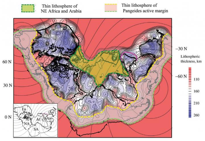
Thick black and magenta lines show northern boundaries of India and Arabia and southern boundary of Eurasian craton. Dashed light-green line marks outer margin of Pangeides active margin. Dashed yellow line shows approximate boundary between active margin and arc of thick lithosphere. Dashed dark-green line outlines area underlain by thinner lithosphere that now underlies North Africa, Arabia, and western Europe. Inset shows same reconstruction without any lithospheric thickness contours. NA–North America;, Eu–Eurasia; SA–South America; Af–Africa; An–Antarctica; Au–Australia. Oblique Mercator projection with axis 30°N, 80°E. Credit: McKenzie et al., Geology, Geological Society of America
Two hundred and fifty million years ago, all the major continents were joined together, forming a continent called Pangea (which means “all land” in Greek). The plate thickness of continents can now be measured using seismology, and it is surprisingly variable, from about 90 km beneath places like California or Western Europe, to more than 200 km beneath the older interiors of the U.S., Eastern Europe, and Russia.
Authors Dan McKenzie, Michael C. Daly, and Keith Priestley wondered what the pattern of plate thickness looked like before Pangea broke up — so they reconstructed Pangea using Rayleigh wave tomography and plate tectonics, taking the plate thickness with the continents as they moved them.
To their surprise, the thick parts of the plates all came together to form a boomerang-shaped arc. The outside of the boomerang consists of a subduction zone where oceanic plates were returned to the mantle. The inside of the boomerang consists of plate with a thickness of about 100 km, which was strongly deformed and heated about 600 million years ago. Pangea itself was assembled from a number of different plates. The continental deformation that took place during this assembly must have been controlled by the plate thickness, since it produced a continuous boomerang shaped region of thick plate.
Reference:
The lithospheric structure of Pangea
Dan McKenzie et al., Bullard Labs, University of Cambridge, Cambridge, UK. Published online ahead of print on 17 July 2015; DOI: 10.1130/G36819.1.
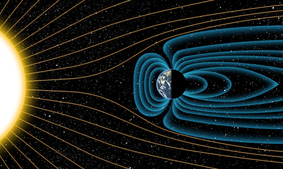
An artist’s depiction of Earth’s magnetic field deflecting high-energy protons from the sun four billion years ago. Note: The relative sizes of the Earth and Sun, as well as the distances between the two bodies, are not drawn to scale. Credit: Graphic by Michael Osadciw/University of Rochester
Since 2010, the best estimate of the age of Earth’s magnetic field has been 3.45 billion years. But now a researcher responsible for that finding has new data showing the magnetic field is far older.
John Tarduno, a geophysicist at the University of Rochester and a leading expert on Earth’s magnetic field, and his team of researchers say they believe the Earth’s magnetic field is at least four billion years old.
“A strong magnetic field provides a shield for the atmosphere,” said Tarduno, “This is important for the preservation of habitable conditions on Earth.”
The findings by Tarduno and his team have been published in the latest issue of the journal Science.
Earth’s magnetic field protects the atmosphere from solar winds–streams of charged particles shooting from the Sun. The magnetic field helps prevent the solar winds from stripping away the atmosphere and water, which make life on the planet possible.
Earth’s magnetic field is generated in its liquid iron core, and this “geodynamo” requires a regular release of heat from the planet to operate. Today, that heat release is aided by plate tectonics, which efficiently transfers heat from the deep interior of the planet to the surface. But, according to Tarduno, the time of origin of plate tectonics is hotly debated, with some scientists arguing that Earth lacked a magnetic field during its youth.
Given the importance of the magnetic field, scientists have been trying to determine when it first arose, which could, in turn, provide clues as to when plate tectonics got started and how the planet was able to remain habitable.
Fortunately for scientists, there are minerals–such as magnetite–that lock in the magnetic field record at the time the minerals cooled from their molten state. The oldest available minerals can tell scientists the direction and the intensity of the field at the earliest periods of Earth’s history. In order to get reliable measurements, it’s crucial that the minerals obtained by scientists are pristine and never reached a sufficient heat level that would have allowed the old magnetic information within the minerals to reset to the magnetic field of the later time.
The directional information is stored in microscopic grains inside magnetite- a naturally occurring magnetic iron oxide. Within the smallest magnetite grains are regions that have their own individual magnetizations and work like a tape recorder. Just as in magnetic tape, information is recorded at a specific time and remains stored unless it is replaced under specific conditions.
Tarduno’s new results are based on the record of magnetic field strength fixed within magnetite found within zircon crystals collected from the Jack Hills of Western Australia. The zircons were formed over more than a billion years and have come to rest in an ancient sedimentary deposit. By sampling zircons of different age, the history of the magnetic field can be determined.
The ancient zircons are tiny–about two-tenths of a millimeter–and measuring their magnetization is a technological challenge. Tarduno and his team used a unique superconducting quantum interference device, or SQUID magnetometer, at the University of Rochester that provides a sensitivity ten times greater than comparable instruments.
But in order for today’s magnetic intensity readings of the magnetite to reveal the actual conditions of that era, the researchers needed to make sure the magnetite within the zircon remained pristine from the time of formation.
Of particular concern was a period some 2.6 billion years ago during which temperatures in the rocks of the Jack Hills reached 475?C. Under those conditions, it was possible that the magnetic information recorded in the zircons would have been erased and replaced by a new, younger recording of Earth’s magnetic field.
“We know the zircons have not been moved relative to each other from the time they were deposited,” said Tarduno. “As a result, if the magnetic information in the zircons had been erased and re-recorded, the magnetic directions would have all been identical.”
Instead, Tarduno found that the minerals revealed varying magnetic directions, convincing him that the intensity measurements recorded in the samples were indeed as old as four billion years.
The intensity measurements reveal a great deal about the presence of a geodynamo at the Earth’s core. Tarduno explains that solar winds could interact with the Earth’s atmosphere to create a small magnetic field, even in the absence of a core dynamo. Under those circumstances, he calculates that the maximum strength of a magnetic field would be 0.6 ?T (micro-Teslas). The values measured by Tarduno and his team were much greater than 0.6 ?T, indicating the presence of a geodynamo at the core of the planet, as well as suggesting the existence of the plate tectonics needed to release the built-up heat.
“There has been no consensus among scientists on when plate tectonics began,” said Tarduno. “Our measurements, however, support some previous geochemical measurements on ancient zircons that suggest an age of 4.4 billion years.”
The magnetic field was of special importance in that eon because solar winds were about 100 times stronger than today. In the absence of a magnetic field, Tarduno says the protons that make up the solar winds would have ionized and stripped light elements from the atmosphere, which, among other things, resulted in the loss of water.
Scientists believe that Mars had an active geodynamo when that planet was formed, but that it died off after four billion years. As a result, Tarduno says, the Red Planet had no magnetic field to protect the atmosphere, which may explain why its atmosphere is so thin.
“It may also be a major reason why Mars was unable to sustain life,” said Tarduno.
Reference:
J. A. Tarduno, R. D. Cottrell, W. J. Davis, F. Nimmo, R. K. Bono. A Hadean to Paleoarchean geodynamo recorded by single zircon crystals. Science, 2015; 349 (6247): 521 DOI: 10.1126/science.aaa9114
Benjamin Gill was part of a team that collected, analyzed, and statistically modeled rock data from across the world.
The discovery, published in the journal Nature, calls into question the long held theory that a dramatic change in oxygen levels might have been responsible for the appearance of complicated life forms like whales, sharks, and squids evolving from less complicated life forms, such as microorganisms, algae, and sponges.
The researchers discovered oxygen levels rose in the water and atmosphere, but at lower levels than was thought necessary to trigger life changes.
“We suggest that about 635 million to 542 million years ago, Earth passed some low, but critical, threshold in oxygenation for animals,” said Benjamin Gill, an assistant professor of geoscience in the College of Science. “That threshold was in the range of a 10 to 40 percent increase, and was the second time in Earth’s history that oxygen levels significantly rose.”
The scientists estimated oxygen levels by analyzing iron found in shale rock, which was once mud on ancient seafloors. The location and amounts of iron in the rock gave important clues about ancient ocean water chemistries over time.
Rock data from across the world were collected by the research team, analyzed, compiled, and statistically modeled.
Many organisms on Earth, including animals, need oxygen to produce energy and perform other life functions.
“Going forward we will need much more precise constraints on the magnitude of oxygenation and the physiological requirements of early animals to continue testing the impact of oxygenation on Cambrian animal life,” said Erik Sperling, an assistant professor of geological and environmental sciences at Stanford University, and first author on the paper.
Reference:
Erik A. Sperling, Charles J. Wolock, Alex S. Morgan, Benjamin C. Gill, Marcus Kunzmann, Galen P. Halverson, Francis A. Macdonald, Andrew H. Knoll, David T. Johnston. Statistical analysis of iron geochemical data suggests limited late Proterozoic oxygenation. Nature, 2015; 523 (7561): 451 DOI: 10.1038/nature14589
If oxygen was a driver of the early evolution of animals, only a slight bump in oxygen levels facilitated it, according to a multi-institutional research team that includes a Virginia Tech geoscientist.
Fossil fish teeth recovered from the ocean floor around Tasmania have shed new light on the origins of the world’s largest ocean current, according to a paper released in Nature this week.
Analysis of fish teeth recovered from drilling of the ocean floor, combined with the study of tectonic plate movements by Dr Joanne Whittaker of the University of Tasmania’s Institute for Marine and Antarctic Studies and Dr Simon Williams from the University of Sydney, has revealed how the flow of water around Antarctica began.
“The Antarctic Circumpolar Current (ACC) is the world’s largest ocean current. It flows clockwise around Antarctica because there are no land masses in the way and it plays a role in maintaining the large ice sheets on Antarctica because it keeps warmer ocean waters away,” Dr Whittaker explained.
“Despite its role in stabilising Antarctic ice sheets, the onset of the Antarctic Circumpolar Current has been poorly understood.
“Tasmania separating from Antarctica about 35 million years ago created the Tasmanian Seaway and for a long time scientists have thought that the opening of this seaway enabled the onset of the ACC, but we’ve found out this is not the case.”
In the paper ‘Onset of Antarctic Circumpolar Current 30 million years ago as Tasmanian Gateway aligned with westerlies’ the Australian scientists and US collaborators, who studied fish teeth in ocean sediment, show that in fact the Tasmanian Seaway had already been open for up to five million years before the ACC became a circulation feature.
“We discovered that opening the Tasmanian Seaway on its own wasn’t enough. It needed to move far enough north to be in the westerly wind band. When the seaway first opened it was too far south. Once it moved further north, the westerly winds were able to drive water through the seaway, and the Earth’s biggest ocean current began,” Dr Whittaker said.
“The ACC is important because it regulates the exchange of heat and carbon between the ocean and the atmosphere and influences vertical ocean structure, deep-water production and the global distribution of nutrients and chemical tracers.”
The US researchers used fossil fish teeth from different layers of sediments deposited on the sea floor to build a record over many millions of years of seawater composition at sites around Tasmania.
Different oceans have distinct chemical (termed isotopic) “fingerprints”, and this difference in the seawater is recorded in fish teeth that settle on the ocean floor, with the isotopes in their teeth preserving the seawater composition at their time of death.
The records show how Tasmania once formed a barrier between Pacific and Indian oceans, but as they moved apart water began to mix, first flowing from the Pacific towards the Indian Ocean, and then from the Indian Ocean to the Pacific, as it still does today.
These changes in ocean circulation are linked to global climate, and scientists believe this may have played a role in the draw down or sinking of carbon dioxide, leading to stabilisation of the ‘icehouse’ world.
Reference:
Howie D. Scher, Joanne M. Whittaker, Simon E. Williams, Jennifer C. Latimer, Wendy E. C. Kordesch & Margaret L. Delaney. Onset of Antarctic Circumpolar Current 30 million years ago as Tasmanian Gateway aligned with westerlies. DOI:10.1038/nature14598
Relating the metagenome and metatranscriptome. Genes involved in methanogenesis are color coded by pathway type: CO 2 to methane in green (96 genes), methanol to methane in red (5 genes) and acetate to methane in blue (209 genes). Common genes, shared between pathway types, are yellow (80 genes). In the background is a two-dimensional density estimation for all 250,596 genes Credit: Bremges et al. GigaScience 2015 4:33 doi:10.1186/s13742-015-0073-6
New research in the Open Access journal GigaScience presents a virtual package of data for biogas production, made reusable in a containerized form to allow scientists to better understand the production of biofuels.
One of the promising areas in biofuels development is biogas, which has huge potential as a renewable and clean source of energy. Biogas is the production of methane gas through the anaerobic digestion (fermentation) of organic matter such as agricultural or food waste. Detailed knowledge on the functioning of the fermentation process is key for optimizing this process; however, the vast majority of the microbes involved remain unknown and cannot be cultivated in laboratories.
In new research just published in the Open Access journal GigaScience, researchers from Bielefeld University in Germany have now characterized the complex communities of micro-organisms in a biogas plant that generates heat and power from maize silage and pig manure. Further, the authors took an unusual step to make their research more reproducible by creating a virtual ‘container’ of their data and tools.
For their study, the researchers carried out metagenomic and meta-transcriptomic analyses, which resulted in the generation of DNA and RNA sequences from the thousands of microbial species present. From this they were able to create a catalogue of 250,000 genes that enabled the researchers to begin defining the underlying biology of methane production. While this data production only scratches the surface of the vast amount of information gathered, the authors furthered the usefulness of this resource by releasing all of the data and computational methods as a shareable container. These containers enable others, at the press of a few buttons, to execute the same analyses in the cloud. This not only makes the research reproducible, but also allows researchers around the world to build on these resources to more rapidly delineate the important processes involved in biogas generation and to better explore its use for biofuel.
As experiments become more data-intensive, reviewing and publishing the methods and results of scientific studies become increasingly challenging. To get around this, the authors used the rapidly emerging Docker platform, which effectively wraps software in a system that includes everything needed to rerun it. This removes the need for other researchers to install and maintain the many complex bioinformatics tools and software libraries: something that can be very technically challenging for researchers without the computational resources and skills.
“We decided to use virtualisation techniques to encapsulate our analysis workflow and make it basically independent from the host it is executed on” says Andreas Bremges, first author of the study. Peter Belmann built the Docker container for the biogas study, and is a core team member of the bioboxes project to standardize interchangeable bioinformatics software containers.
“The reproducibility of published research is an important aspect of science,” highlights Peter Li, Lead Data Manager at GigaScience, who undertook the step of exactly recreating the results in the paper, which is extremely unusual in any other scientific publication. “Andreas and his colleagues provided a Docker container that encapsulated the method used to process the data from their biogas study. This made my job of checking the reproducibility of their results much easier as their Docker container took care of installing the bioinformatics tools and their dependencies on my cloud server”.
The use of Docker in this “container” publication is a step towards moving publishing away from static and often un-reproducible papers –which have changed little since the 17th century– to more reproducible digital objects that better fit 21st century technology.
Reference:
1. Bremges, A., Maus, I., Belmann, P., Eikmeyer, F., Winkler, A., Albersmeier, A., Puhler, A., Schluter, A., Sczyrba, A.: (2015) Deeply sequenced metagenome and metatranscriptome of a biogas-producing microbial community from an agricultural production-scale biogas plant. GigaScience 4:33 DOI:10.1186/s13742-015-0073-6
2. Bremges, A., Maus, I., Belmann, P., Eikmeyer, F., Winkler, A., Albersmeier, A., Puhler, A., Schluter, A., Sczyrba, A.: Supporting data and materials for “Deeply sequenced metagenome and metatranscriptome of a biogas-producing microbial community from an agricultural production-scale biogas plant”. GigaScience
The Nalunaq Gold Mine contains hanging wall rocks (pictured) which are Paleoproterozoic amphibolite-facies metadolerites. Credit: James St. John
GOLD has been found in geologically unusual circumstances about 250km east of Carnarvon on the margin of the Japan-sized former continent which forms part of the Gascoyne.The gold deposit is found along the margin where two tectonic plates, the Yilgarn Craton and Glenburgh Terrane, collided about two billion years ago.
The Glenburgh Terrane later became trapped between the Yilgarn and Pilbara Cratons, thereby forming a single tectonic plate.
Geological Survey of Western Australia geologist Lisa Roche says the ore is classed as upper amphibolite to granulite facies, which means it has been exposed to a massive seven to 10 kilobars of pressure and temperatures of 500-1000 degrees Celcius.
“Gold deposits in upper amphibolite to granulite facies rocks are quite rare,” she says.
“Known examples commonly attract debate as to whether they actually formed at these high pressures and temperatures or instead were formed early and subsequently metamorphosed or formed late and after peak metamorphism.”
Ms Roche, who has been studying the formation as part of the Geological Survey Masters Program, says the gold had almost certainly been deposited before the tectonic plates met.
She came to this conclusion after nine months of field mapping, visual drill core logging, thin-section petrography and analysis of the microstructure of the gold grains themselves.
“We looked at the internal structure of the gold itself and we found features that suggested it had been through post depositional processes such as deformation, metamorphism or weathering,” she says.
Low silver levels suggest formation processes
Those features included low silver levels of one to three per cent in the gold, whereas gold typically contains five to 20 per cent silver when it first crystallises.
“We could see the gold itself was actually made up of several smaller gold grains, and in between these gold grains there were high purity gold veinlets,” she says.
“They form when silver’s being leached from the gold and removed along the grain boundaries.”
She says this showed the gold had been deformed or metamorphosed.
They also found well-rounded inclusions of pyrrhotite, a sulfide commonly associated with gold mineralising fluids.
“We’ve interpreted this as a peak metamorphic mineral, so that suggested a sulfide phase was present in the host rock before the peak of metamorphism,” she says.
“These observations all have suggested to us that the gold mineralising event occurred before the peak metamorphism.”
As the rocks metamorphosed when the plates collided she says they concluded the gold must be even older.
Note: The above post is reprinted from materials provided by ScienceNetwork WA. The original article was written by Geoff Vivian.