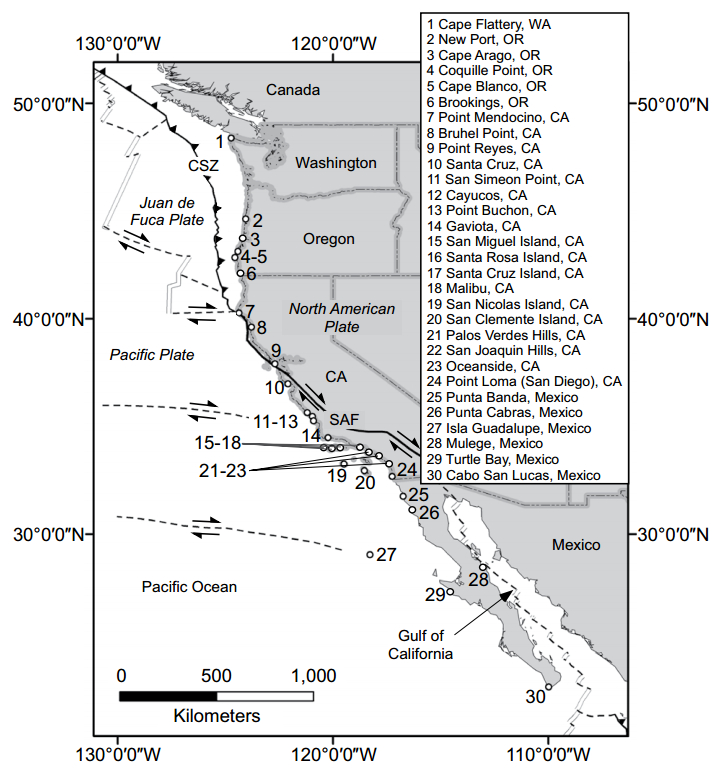
This is a map showing the locations mentioned in the text as well as the major tectonic features of the Pacific coast of North America. CA — California, SAF — San Andreas fault, CSZ — Cascadia subduction zone. Credit: GSA Bulletin and Simms et al.
A new GSA Bulletin study shows that uplift rates across the Pacific Coast of the USA and northern Mexico have been overestimated by an average of more than 40%. These lower uplift rates imply that the shorelines of the West Coast are rising at a slower rate than previously thought, and this may have important implications for coastal management, including earthquake hazards and the potential impact of sea-level rise to coastlines across the Pacific Coast.
In their paper for GSA Bulletin, Alexander Simms and colleagues write, “Factors other than tectonics contribute to local sea-level change, and one important, yet often overlooked, contribution is the earth-ocean response to the changing distribution of surface loads of ice and water, often referred to as … glacial isostatic adjustment. Neglect of this effect, particularly along coastal sections at variable distances from the former ice sheets, such as the eastern Pacific coast from northern Mexico to the U.S.-Canada border, introduces large errors in uplift estimates.”
Reference:
Marine terraces and rates of vertical tectonic motion: The importance of glacio-isostastic adjustment along the Pacific Coast of central North America
A.R. Simms et al., University of California, Santa Barbara, California, USA. Published online ahead of print on 29 July 2015; DOI: 10.1130/B31299.1.
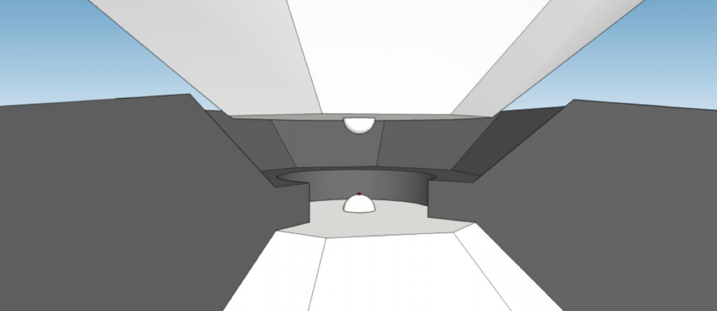
This is a schematic of the pressure chamber of the double-stage diamond anvil cell: The osmium sample is just 3 microns small and sits between two semi-balls made of nanocristalline diamond of extraordinary strength. Credit: Elena Bykova/University of Bayreuth
An international team of scientists led by the University of Bayreuth and with participation of DESY has created the highest static pressure ever achieved in a lab: Using a special high pressure device, the researchers investigated the behaviour of the metal osmium at pressures of up to 770 Gigapascals (GPa) – more than twice the pressure in the inner core of the Earth, and about 130 Gigapascals higher than the previous world record set by members of the same team. Surprisingly, osmium does not change its crystal structure even at the highest pressures, but the core electrons of the atoms come so close to each other that they can interact – contrary to what is usually known in chemistry. This fundamental result published in the journal Nature has important implications for understanding physics and chemistry of highly compressed matter, for design of materials to be used at extreme conditions, and for modelling the interiors of giant planets and stars.
Metallic osmium (Os) is one of the most exceptional chemical elements, having at ambient pressure the highest known density of all elements, one of the highest cohesive energies, melting temperatures, and a very low compressibility – it is almost as incompressible as diamond. Due to its hardness, osmium finds applications in alloys used for instance as electrical contacts, wear-resistant machine parts and tips for high-quality ink pens.
“High pressure is known to radically affect properties of chemical elements: metals like sodium may become transparent insulators; gases like oxygen solidify and become electrical conductors – and even superconductors,” explains Natalia Dubrovinskaia from the University of Bayreuth, together with Leonid Dubrovinsky the main author of the study. “as any other material subjected to very high compression, osmium is expected to change its crystal structure.”
For their experiments, the scientists used a device for generating ultra-high static pressures developed by Dubrovinsky and Dubrovinskaia at Bayreuth. The device uses micro-anvils of only 10 to 20 micrometres (a micrometre is a thousandths of a millimetre) in diameter which are made of nanocrystalline diamond. These nanocrystals, which are diamond grains of a nano-size, are bound together forming a bulk micro-anvil. The many grain boundaries make the nanocrystalline anvils even harder than single crystal diamonds, extending the range of static pressure in experiments from about 400 GPa to 770 GPa at room temperature.
For probing the samples under these extreme conditions, the team used high-brilliance X-rays from the synchrotron sources PETRA III at DESY, ESRF in France and APS in the U.S. The team found out that Osmium shows unprecedented structural stability and keeps its crystal structure even at huge pressures of about 770 GPa.
While the volume of the osmium unit cell steadily shrinks with rising pressure, very accurate X-ray diffraction experiments revealed anomalies in the behaviour of the lattice parameters describing the unit cell. Usually, changes in materials properties under pressure are associated with modifications in the configurations of the outer (valence) electrons. But in case of highly compressed osmium the reason for the observed structural anomaly is an interaction between the inner (core) electrons, as suggested by state-of-the-art theoretical calculations. “This work demonstrates that ultra-high static pressures can force the core electrons to interplay,” explains Dubrovinsky. “The ability to affect the core electrons even in such incompressible metals as osmium in static high-pressure experiments opens up exciting opportunities in searching for new states of matter.”
The experiments pave the way for investigating materials under conditions of the inner core of giant planets. “In the last 20 years, astronomers found more than thousand planets around other stars, nearly all of them bigger than our Earth,” says co-author Hanns-Peter Liermann from DESY, responsible for the beamline P02 at PETRA III, where some of the experiments took place. “With the newly developed double-stage diamond anvil cell and with the very focused high intensity X-ray spot at PETRA III – or later at the X-ray laser European XFEL that is currently being constructed in the Hamburg area – we can probe a variety of rocky planet compositions under most extreme conditions and will learn a lot about the composition and evolution of such planets.”
Reference:
The most incompressible metal osmium at static pressures above 750 GPa; L. Dubrovinsky, N. Dubrovinskaia, E. Bykova, M. Bykov, V. Prakapenka, C. Prescher, K. Glazyrin, H.-P. Liermann, M. Hanfland, M. Ekholm, Q. Feng, L. V. Pourovskii, M. I. Katsnelson, J. M. Wills, and I. A. Abrikosov; „Nature”, 2015; DOI: 10.1038/nature14681
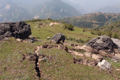
Large ground cracks on a small ridge and landslide in the background after the Nepal quake of April 2015, upper Bhote Koshi river valley. Credit: O. Marc, GFZ
In mountainous regions earthquakes often cause strong landslides, which can be exacerbated by heavy rain. However, after an initial increase, the frequency of these mass wasting events, often enormous and dangerous, declines, in fact independently of meteorological events and aftershocks. These new findings are presented by a German-Franco-Japanese team of geoscientists in the current issue of the journal Geology, under the lead of the GFZ German Research Centre for Geosciences. Even after strong earthquake the activity of landslides returns back over the course of one to four years to the background level before the earthquake.
The interactions over time between earthquakes and processing shaping the landscape are still not well understood. The geoscientists have investigated areas affected by landslides related to four moderate to severe earthquakes (6.6 to 7.6 on Richter scale). “The main difficulty was that one must distinguish between the meteorological and the seismic causes of landsliding. Heavy rain can also produce landslides and can enhance landsliding after an earthquake,” says GFZ scientists Marc Odin, the lead author of the study. Two processes are interacting here. A strong earthquake shakes soil layer loose from the underlying bedrock and also damages the rock below the top soil. Water seeps into the resulting the cracks and crevices and acts like a lubricating film on which a mountain slope slides into the valley.
With the present results of the team of geoscientists, this conceptual model has to be modified. “We analytically separated the effect of the rain from the seismic activity and so were able to determine that the decrease of landslides through time is based on an internal healing process of the landscape,” said Marc Odin. The destabilization of the landscape caused by the quake gradually recovers. In the course of months to years, depending on weather, rocks and the strength of the earthquake, the slide rates return to the pre-earthquake level: The cracks slowly get closed again or are filled with sand and earth. The landscape self-heals its underlayer and returns to its background hazard potential.
This research is highly relevant: currently the GFZ analyzes these processes in the context of the Nepal-quake of April this year: “We had the chance to start a series of measurements directly after the quake and continue for the next few years,” explained Niels Hovius, Head of the Section “Geomorphology” at the GFZ, about the current deployment of his team in the Himalayas.
Reference:
O. Marc, N. Hovius, P. Meunier, T. Uchida, S. Hayashi. Transient changes of landslide rates after earthquakes. Geology, 2015; G36961.1 DOI: 10.1130/G36961.1
A melting tongue of Exit Glacier near Seward, Alaska, continues to dwindle and pour water into streams below, as it has been doing for decades. Credit: Photo courtesy of Oregon State University
A recalculation of the dates at which boulders were uncovered by melting glaciers at the end of the last Ice Age has conclusively shown that the glacial retreat was due to rising levels of carbon dioxide and other greenhouse gases, as opposed to other types of forces.
Carbon dioxide levels are now significantly higher than they were at that time, as a result of the Industrial Revolution and other human activities since then. Because of that, the study confirms predictions of future glacial retreat, and that most of the world’s glaciers may disappear in the next few centuries.
The findings were published today in Nature Communications by researchers from Oregon State University, Boston College and other institutions. They erase some of the uncertainties about glacial melting that had been due to a misinterpretation of data from some of these boulders, which were exposed to the atmosphere more than 11,500 years ago.
“This shows that at the end of the last Ice Age, it was only the increase in carbon dioxide and other greenhouse gases that could have caused the loss of glaciers around the world at the same time,” said Peter Clark, a professor in the OSU College of Earth, Ocean and Atmospheric Sciences, and co-author on the study.
“This study validates predictions that future glacial loss will occur due to the ongoing increase in greenhouse gas levels from human activities,” Clark said. “We could lose 80-90 percent of the world’s glaciers in the next several centuries if greenhouse gases continue to rise at the current rate.”
Glacial loss in the future will contribute to rising sea levels and, in some cases, have impacts on local water supplies.
As the last Ice Age ended during a period of about 7,000 years, starting around 19,000 years ago, the levels of carbon dioxide in the atmosphere increased from 180 parts per million to 280 parts per million. But just in the past 150 years, they have surged from 280 to about 400 parts per million, far higher than what was required to put an end to the last Ice Age.
The new findings, Clark said, were based on a recalculation of the ages at which more than 1,100 glacial boulders from 159 glacial moraines around the world were exposed to the atmosphere after being buried for thousands of years under ice.
The exposure of the boulders to cosmic rays produced cosmogenic nuclides, which had been previously measured and used to date the event. But advances have been made in how to calibrate ages based on that data. Based on the new calculations, the rise in carbon dioxide levels — determined from ancient ice cores -matches up nicely with the time at which glacial retreat took place.
“There had been a long-standing mystery about why these boulders were uncovered at the time they were, because it didn’t properly match the increase in greenhouse gases,” said Jeremy Shakun, a professor at Boston College and lead author on the study. “We found that the previous ages assigned to this event were inaccurate. The data now show that as soon as the greenhouse gas levels began to rise, the glaciers began to melt and retreat.”
There are other forces that can also cause glacial melting on a local or regional scale, the researchers noted, such as changes in the Earth’s orbit around the sun, or shifts in ocean heat distribution. These factors probably did have localized effects. But the scientists determined that only the change in greenhouse gas levels could have explained the broader global retreat of glaciers all at the same time.
In the study of climate change, glaciers have always been of considerable interest, because their long-term behavior is a more reliable barometer that helps sort out the ups-and-downs caused by year-to-year weather variability, including short-term shifts in temperature and precipitation.
Other collaborators on this research were from the University of Wisconsin, Purdue University, and the National Center for Atmospheric Research. The work was supported by the National Oceanic and Atmospheric Administration and the National Science Foundation.
Reference:
Jeremy D. Shakun, Peter U. Clark, Feng He, Nathaniel A. Lifton, Zhengyu Liu, Bette L. Otto-Bliesner. Regional and global forcing of glacier retreat during the last deglaciation. Nature Communications, 2015; 6: 8059 DOI: 10.1038/ncomms9059
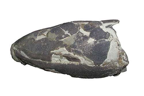
One of the original skulls used in the project. Credit: Dr Laura Porro
A new bone in the skull of an iconic fossil animal that represents the ‘missing link’ between fish and all land-dwelling vertebrate animals has been found by researchers from the University of Bristol.
Dr Laura Porro and colleagues in Bristol’s School of Earth Sciences and at the University of Cambridge applied high-resolution X-ray computed tomography (CT) scanning to several specimens of Eusthenopteron. This prehistoric fish grew up to 1.8 metres (6 feet) in length and patrolled shallow lagoons 385 million years ago during the Late Devonian period.
The researchers used cutting-edge software to digitally strip away rock from fossil bone and separate individual bones and teeth from each other. The aim of the study was to better understand the lower jaw of Eusthenopteron, which had never been fully described. As they ‘digitally dug’ deeper, however, researchers found a surprise in the shape of a new jaw bone.
Eusthenopteron is what is known as a lobe-finned fish and is important in evolutionary terms as it is related to the first tetrapods. Tetrapods are the four-footed vertebrates that took their first steps on land nearly 20 million years later during one of the great transitions in the history of life.
It is crucial for understanding why vertebrates moved out of water and onto land in the first place. The fossil is not new to science and was first described in 1881. Since its initial description, thousands of specimens have been discovered, making it one of the best known fossil fish.
Lead author, Dr Porro, now at the Royal Veterinary College (RVC), said: “While examining CT scans of multiple specimens of Eusthenopteron, we kept finding a long, thin bone near the front of the lower jaw that we could not identify. It just isn’t one of the ‘standard’ bones that make up the lower jaws of either lobe-finned fish or tetrapods.”
It turned out that the structure had been noticed in other species of lobe-finned fish and tetrapods, but was assumed to be either a broken fragment or an extension of surrounding bones. In fact, CT scans demonstrate it represents a bone entirely new to science, which the authors of the study have called the ‘postsymphysial’ because it occurs immediately behind (‘post’) the area where the right and left halves of the lower jaw come together (‘symphysis’).
While the bone occurs in several other lobe-finned fish and tetrapods, its presence in the lower jaw was short-lived. “By the time tetrapods made their final move onto land at the end of the Devonian and beginning of the Carboniferous, the postsymphysial disappears,” Dr Porro added.
Additionally, the study found new clues to how Eusthenopteron captured its prey. Earlier studies suggested that because of its strong, fish-like appearance, Eusthenopteron captured its prey the way most modern fish do – using suction. The size and distribution of its teeth and the shape of contacts between individual bones, however, suggest it may have also used a strong bite to tackle larger prey.
The researchers are applying these methods to other early tetrapods to learn more about their anatomy and ecology. Digital models are also useful for education and scientific research, as they can be easily accessed by people around the world.
Reference:
“Computed tomography, anatomical description and three-dimensional reconstruction of the lower jaw of Eusthenopteron foordi Whiteaves, 1881 from the Upper Devonian of Canada.” Palaeontology. DOI: 10.1111/pala.12192
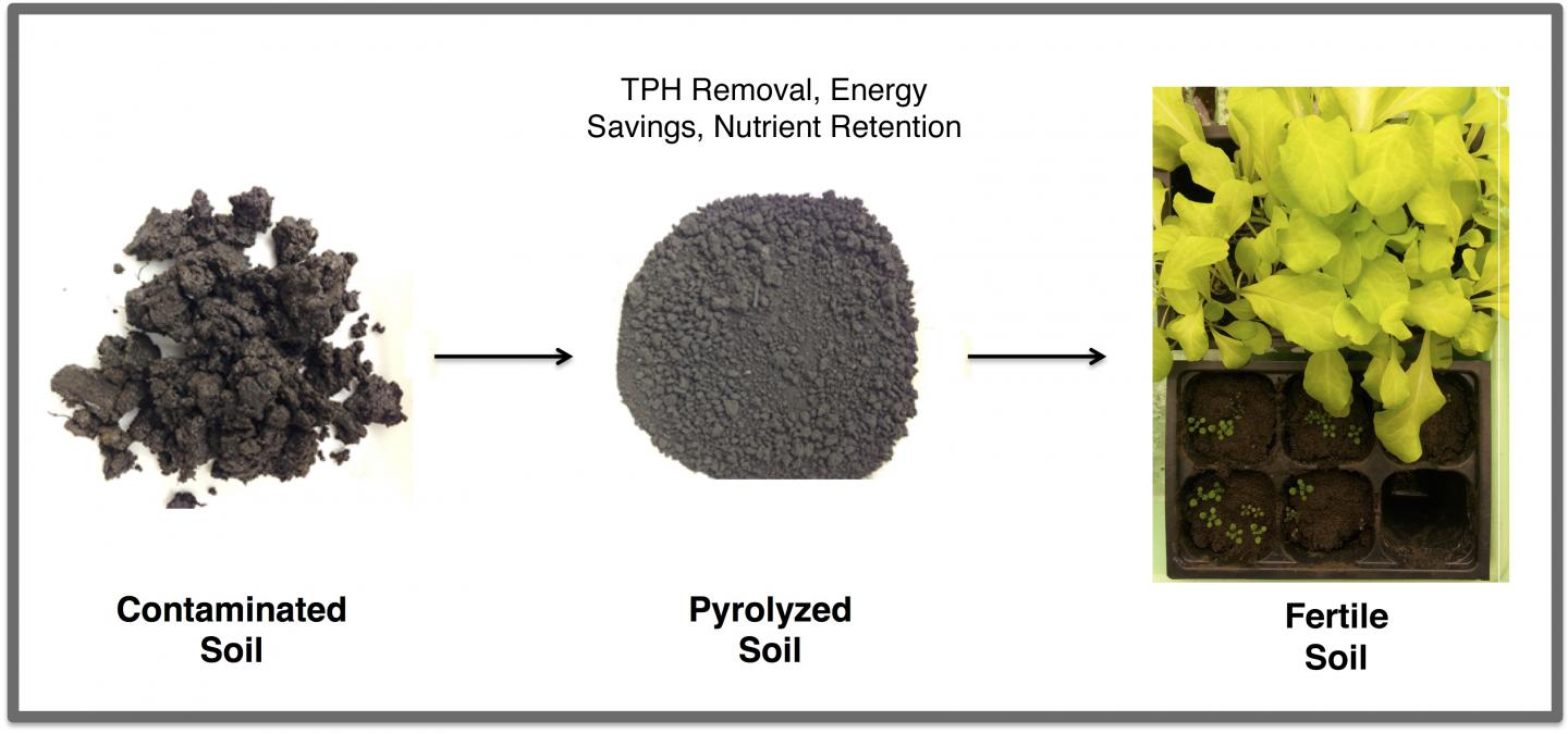
Rice University pyrolyzed oil-contaminated soil to reduce total petroleum hydrocarbons below federal standards, while leaving beneficial carbons in the soil. The lab grew lettuce in samples of reclaimed soil to test its viability. Credit: Julia Vidonish/Rice University
Rice University scientists are cleaning soil contaminated by oil spills in a way that saves energy and reclaims the soil’s fertility.
They use a process known as pyrolysis, which involves heating contaminated soils in the absence of oxygen. This approach is much better for the environment than standard incineration techniques for fast remediation, said Rice environmental engineer Pedro Alvarez.
“Our original goal was to speed the response to oil spills, but our aspiration was to turn contaminated soil into fertile soil,” said Alvarez, the George R. Brown Professor and chair of Rice’s Civil and Environmental Engineering Department.
The new paper by Alvarez and his Rice colleagues in the American Chemical Society journal Environmental Science and Technology demonstrates how they’ve done just that.
Off-shore oil spills tend to get the most attention, Alvarez said, but 98 percent of spills – more than 25,000 per year — occur on land. Industry and governments worldwide spend more than $10 billion annually to clean up oil spills.
The Rice team found that pyrolyzing contaminated soil for three hours not only reduced the amount of petroleum hydrocarbons left to well below regulatory standards (typically less than 0.1 percent by weight), but also enhanced the soil’s fertility by turning the remaining carbon into beneficial char.
“We initially thought we could turn the hydrocarbons into biochar,” Alvarez said. “We turned out to be partly wrong: We didn’t get biochar, but [we got] a carbonaceous material that we call char and resembles coke.
“But we were correct in thinking that by removing toxic pollutants and the hydrophobicity that repels water that plants need, and by retaining some of the carbon and perhaps some of the nutrients, we would enhance plant growth,” he said.
The researchers proved that by successfully growing lettuce in reclaimed soil in the lab. “There’s no one plant officially accepted as the standard for testing petroleum toxicity, but lettuce has been accepted by the community as very sensitive to toxins, especially petroleum,” said Rice graduate student Julia Vidonish, the paper’s lead author. “Reclaimed soil may not necessarily be used to grow food, but it certainly could be used for re-greening: planting grass to minimize erosion and to restore vegetation,” Alvarez said.
“Our process is part thermal desorption, but it takes advantage of petroleum chemistry,” said Rice chemical engineer and co-author Kyriacos Zygourakis. “By heating the contaminated soils to about 420 degrees Celsius in the absence of oxygen, we first drive out the lighter hydrocarbons. That’s the desorption part. But when the temperature gets above 350 degrees, the high-molecular-weight hydrocarbons, the resins and asphaltenes, undergo a series of cracking and condensation reactions to form solid char, similar to the petroleum coke produced in refineries.
“We leave some of the hydrocarbons in the treated soil but in a solid, more benign form,” he said. “The Environmental Protection Agency does not classify petroleum coke as hazardous waste. If, on the other hand, you want to remove everything, you have to raise the temperature even higher and introduce oxygen to incinerate the char. But you destroy the soil and use 40 to 60 percent more energy.”
The char produced by pyrolyzing oil-soaked soil is different from biochar, Rice biogeochemist and co-author Caroline Masiello said. Where biochar is a particle unto itself, the coke-like char appears to coat existing soil particles.
“Biochar is a particle that is separate from the soil’s mineral grains,” she said. “It has an internal physical structure that allows it to hold water and nutrients and provides a home for microbes, but here, we’re not making any of those things. We’re making an organic film that coats the minerals.”
Vidonish said the process is scalable and should work with existing remediation equipment. “Incineration and thermal desorption are established technologies, and while this is different, there are similarities,” she said. “We expect companies can take a mobile, field-scale thermal desorption unit and make a couple of modifications to do pyrolysis.”
“We proved we can remove all the bad actors and all the contaminants and at the same time have a final product with agricultural value,” Zygourakis said. “We don’t just turn it into desert sand.”
Much work remains to optimize the process, Vidonish said. “Moving forward, we want to understand how the pyrolysis time and the temperature affect the quality of the char in the soil,” she said.
Reference:
Julia E. Vidonish , Kyriacos Zygourakis , Caroline A. Masiello , Xiaodong Gao , Jacques Mathieu , and Pedro J. J. Alvarez. Pyrolytic Treatment and Fertility Enhancement of Soils Contaminated with Heavy Hydrocarbons. DOI: 10.1021/acs.est.5b02620
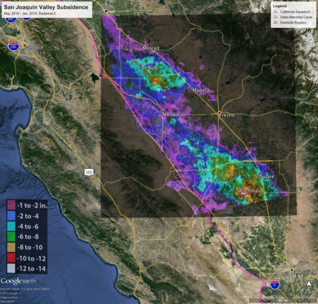
Total subsidence in California’s San Joaquin Valley for the period May 3, 2014 to Jan. 22, 2015, as measured by Canada’s Radarsat-2 satellite. Two large subsidence bowls are evident, centered on Corcoran and south of El Nido. Credit: Canadian Space Agency/NASA/JPL-Caltech
As Californians continue pumping groundwater in response to the historic drought, the California Department of Water Resources has released a new NASA report showing land in the San Joaquin Valley is sinking faster than ever before, nearly 2 inches (5 centimeters) per month in some locations.
“Because of increased pumping, groundwater levels are reaching record lows — up to 100 feet (30 meters) lower than previous records,” said Department of Water Resources Director Mark Cowin. “As extensive groundwater pumping continues, the land is sinking more rapidly and this puts nearby infrastructure at greater risk of costly damage.”
Sinking land, known as subsidence, has occurred for decades in California because of excessive groundwater pumping during drought conditions, but the new NASA data show the sinking is happening faster, putting infrastructure on the surface at growing risk of damage.
NASA obtained the subsidence data by comparing satellite images of Earth’s surface over time. Over the last few years, interferometric synthetic aperture radar (InSAR) observations from satellite and aircraft platforms have been used to produce maps of subsidence with approximately centimeter-level accuracy. For this study, JPL researchers analyzed satellite data from Japan’s PALSAR (2006 to 2010); and Canada’s Radarsat-2 (May 2014 to January 2015), and then produced subsidence maps for those periods. High-resolution InSAR data were also acquired along the California Aqueduct by NASA’s Uninhabited Aerial Vehicle Synthetic Aperture Radar (UAVSAR) (2013 to 2015) to identify and quantify new, highly localized areas of accelerated subsidence along the aqueduct that occurred in 2014. The California Aqueduct is a system of canals, pipelines and tunnels that carries water collected from the Sierra Nevada Mountains and Northern and Central California valleys to Southern California.
Using multiple scenes acquired by these systems, the JPL researchers were able to produce time histories of subsidence at selected locations, as well as profiles showing how subsidence varies over space and time.
“This study represents an unprecedented use of multiple satellites and aircraft to map subsidence in California and address a practical problem we’re all facing,” said JPL research scientist and report co-author Tom Farr. “We’re pleased to supply the California DWR with information they can use to better manage California’s groundwater. It’s like the old saying: ‘you can’t manage what you don’t measure’.”
Land near Corcoran in the Tulare basin sank 13 inches (33 centimeters) in just eight months — about 1.6 inches (4 centimeters) per month. One area in the Sacramento Valley was sinking approximately half-an-inch (1.3 centimeters) per month, faster than previous measurements.
Using the UAVSAR data, NASA also found areas near the California Aqueduct sank up to 12.5 inches (32 centimeters), with 8 inches (20 centimeters) of that occurring in just four months of 2014.
“Subsidence is directly impacting the California Aqueduct, and this NASA technology is ideal for identifying which areas are subsiding the most in order to focus monitoring and repair efforts,” said JPL research scientist and study co-author Cathleen Jones. “Knowledge is power, and in this case knowledge can save water and help the state better maintain this critical element of the state’s water delivery system.” UAVSAR flies on a C-20A research aircraft based at NASA’s Armstrong Flight Research Center facility in Palmdale, California.
The increased subsidence rates have the potential to damage local, state and federal infrastructure, including aqueducts, bridges, roads and flood control structures. Long-term subsidence has already destroyed thousands of public and private groundwater well casings in the San Joaquin Valley. Over time, subsidence can permanently reduce the underground aquifer’s water storage capacity.
“Groundwater acts as a savings account to provide supplies during drought, but the NASA report shows the consequences of excessive withdrawals as we head into the fifth year of historic drought,” Director Cowin said. “We will work together with counties, local water districts, and affected communities to identify ways to slow the rate of subsidence and protect vital infrastructure such as canals, pumping stations, bridges and wells.”
NASA will also continue its subsidence monitoring, using data from the European Space Agency’s recently launched Sentinel-1 mission to cover a broader area and identify more vulnerable locations.
DWR also completed a recent land survey along the Aqueduct — which found 70-plus miles (113-plus kilometers) in Fresno, Kings and Kern counties sank more than 1.25 feet (0.4 meters) in two years — and will now conduct a system-wide evaluation of subsidence along the California Aqueduct and the condition of State Water Project facilities. The evaluation will help the department develop a capital improvement program to repair damage from subsidence. Past evaluations found that segments of the Aqueduct from Los Banos to Lost Hills sank more than 5 feet (1.5 meters) since construction.
NASA and the Indian Space Research Organisation are jointly developing the NASA-ISRO Synthetic Aperture Radar (NISAR) mission. Targeted to launch in 2020, NISAR will make global measurements of the causes and consequences of land surface changes. Potential areas of research include ecosystem disturbances, ice sheet collapse and natural hazards. The NISAR mission is optimized to measure subtle changes of Earth’s surface associated with motions of the crust and ice surfaces. NISAR will improve our understanding of key impacts of climate change and advance our knowledge of natural hazards.
The report, Progress Report: Subsidence in the Central Valley, California, prepared for DWR by researchers at NASA’s Jet Propulsion Laboratory, Pasadena, California, is available at: http://water.ca.gov/groundwater/docs/NASA_REPORT.pdf (14 MB)
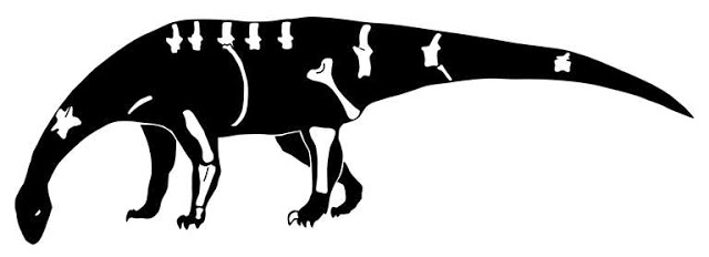
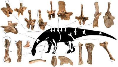
Wits PhD student Blair McPhee has described a new species of dinosaur in a paper to be published in Scientific Reports on 19 September 2015. The new dinosaur, named Pulanesaura eocollum, means the “Rain lizard”.
According to the authors of the paper – McPhee, Dr Matthew Bonnan (Stockton University), Dr Jonah Choiniere (Evolutionary Studies Institute at Wits), Dr Adam Yates (Scientist at the Museum of Central Australia) and Dr Johann Neveling (Geologist from the Council of Geoscience, SA), Pulanesaura was an early member of the long-necked sauropod lineage of dinosaurs, famously represented by Brontosaurus.
Eating habits
The researchers says that the specialised teeth, vertebrae, and forelimb of Pulanesaura was an indication that the new species would have spent all of its time on all fours, browsing lower vegetation. This novel feeding strategy would have resulted in a more energetically conservative feeding posture for Pulanesaura.
This is unlike more primitive prosauropod (scientifically referred to as “basal sauropodomorph”) dinosaurs, which still relied on the forelimb to aid in gathering food from across a broad range of the forest canopy.
Early sauropods like Pulanesaura are incredibly rare in the fossil record, with only a handful of good sauropod specimens known from the Early Jurassic, a time period between 200 and 180 million years ago, when Pulanesaura would have lived.
Much more common at that time in South Africa were bipedal or semi-bipedal sauropodomorph dinosaurs like Massospondylus and Antetonitrus. This might have been because the unique feeding strategy of Pulanesaura restricted the number of lower-browsing dinosaurs that the early Jurassic landscape could have supported.
“This dinosaur showcases the unexpected diversity of locomotion and feeding strategies present in South Africa 200 million years ago. This has serious implications for how dinosaurs were carving up their ecosystems,” says McPhee.
“We used to think that only two species of sauropodomorph dinosaur were present in South Africa. Now we know that the picture was much more complicated, with lots of species present. But Pulanesaura is still special because it was doing something that all these newly discovered species weren’t,” says Choiniere.
Pulanesaura description
Pulanesaura was relatively small (for a sauropod), at about eight metres in length, two metres at the hips, and 5 tonnes in body mass.
Unlike its bipedal ancestors, who used the forelimb as an additional means of gathering food, Pulanesaura would have had to rely on the flexibility of its long neck alone.
Flexibility in the neck meant that the forelimb of Pulanesaura was able to shift to a position entirely beneath the body, thus better supporting the weight of the animal.
Modifications of the neck may have also meant that it would not have needed to move its body about as much to feed – and less movement means less energy expended. This method of feeding was taken to extreme lengths by all gigantic sauropod species.
Bonnan adds, “The traditional picture of sauropod evolution is that when they came onto the scene, the other sauropodomorphs were pushed aside. Pulanesaura turns this notion on its head. Sauropod evolution was occurring alongside and influenced by competition with their sauropodomorph brethren.”
History of the name
The fossils of Pulanesaura were found at Heelbo, a farm in the Eastern Free State where two other recently described South African dinosaur species also come from – Aardonyx and Arcusaurus, both more primitive members of the same lineage.
The late Naude Bremer, former owner of Heelbo, was a strong proponent of palaeontology on his farm. “Pulane” was the childhood Sesotho nickname of Bremer’s daughter, Panie.
Roughly translated, “Pulane” means “comes with rain,” and Pulanesaura was excavated during a particularly rainy period on the property.
These species, along with limb bones of a small predatory dinosaur, the teeth of a huge predatory dinosaur and other bones of as-yet-unknown dinosaurs make Heelbo one of the richest dinosaur localities in southern Africa.
Yates, who excavated the fossil, believes that Heelbo Farm was different from the rest of South Africa 200 million years ago when Pulanesaura was alive.
“The dinosaur fossils we see at Heelbo are different from the typical South African Early Jurassic species and they might have been living in a rare habitat different than the drier ones favoured by famous species like Massospondylus,” he says.
Neveling says what makes Heelbo unique is the fact that unlike the majority of localities of this age which represent dry flood plains, its geology is characterised by a dense concentration of river channel deposits.
“Similar to modern arid environments, the river banks would have supported much denser vegetation that would have provided plenty of food to budding giants,” Neveling adds.
Reference:
“A new basal sauropod from the pre-Toarcian Jurassic of South Africa: evidence of niche-partitioning at the sauropodomorph–sauropod boundary?” Scientific Reports 5, Article number: 13224 (2015) DOI: 10.1038/srep13224
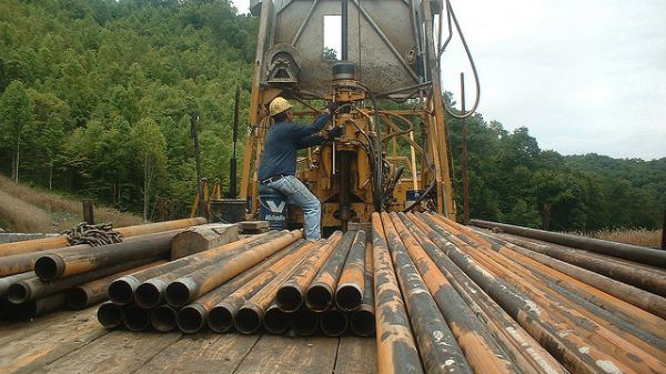
The deposit’s owner, Abra Mining, provided the researchers with drill cores from which they sampled mineralised zones. Credit: Josh “Flickr”
GEOLOGISTS have used a technique developed at Curtin University to determine magmatic fluids came up from the earth’s mantle repeatedly over the past 1600 million years, depositing minerals along a fault line in the Gascoyne region.
Geological Survey of Western Australia researcher Dr Simon Johnson told the Geological Survey Open Day earlier this year the fault had been active 1600, 1375, 1220 and 1000 million years ago.
“Each time that fault gets reactivated there are hydrothermal fluids which percolate through that rock system—they cause alterations and they cause alteration of the ore deposit,” he said.
He said the usual analysis method, by which a rock sample was crushed before analysis, had made it impossible to date when the various minerals present had first been deposited.
However, Professor Birger Rasumussun’s technique, which involves mounting extremely thin slices of rock on a slide, meant small mineral crystals could be identified and individually dated in situ.
Dr Johnson says they applied the technique to a diamond drill core from the Abra deposit.
This is the biggest known mineral deposit in the Capricorn Orogen, which is a deep margin between two former tectonic plates.
He said Abra is a huge lead-zinc deposit, with accessory gold and silver, which is completely covered by younger rocks.
It was detected in a magnetic survey, confirmed by drilling in the early 1980s, and is now a mining lease.
Samples dished up as ultra thin disks
The deposit’s owner, Abra Mining, provided the researchers with drill cores from which they sampled mineralised zones.
Using Prof Rasmussen’s technique they, inspecting them for phosphate minerals like xenotime or monazite which they drilled out as 3mm disks.
They mounted these on tape, encased it in an epoxy glue and placed it in a Sensitive High Resolution Ion Micro Probe (SHRIMP) machine.
This allowed them to fire oxygen ions at the grains of xenotime or the monazite.
The oxygen ions evaporate part of the xenotime or the monazite which they fed into a Faraday collector.
This dated the xenotime grains by measuring various isotope ratios of uranium, thorium, lead and intermediate products.
While it sits at the junction of the former Yilgarn and Pilbara tectonic plates, both of which are rich in minerals, the orogeny has very few working mines.
Dr Johnson said two Curtin University PhD students will apply the new method in an attempt to locate more prospective areas of the orogeny for mineral explorers.
Notes:
Dr Johnson is the Geological Survey of Western Australia’s Proterozoic Orogens Terrane Custodian and Project Manager for the Capricorn Province.
Reference:
Jian-Wei Zi, Birger Rasmussen, Janet R. Muhling, Ian R. Fletcher, Alan M. Thorne, Simon P. Johnson, Huntly N. Cutten, Daniel J. Dunkley, Fawna J. Korhonen. In situ U–Pb geochronology of xenotime and monazite from the Abra polymetallic deposit in the Capricorn Orogen, Australia: Dating hydrothermal mineralization and fluid flow in a long-lived crustal structure. DOI: 10.1016/j.precamres.2015.01.010
Note: The above post is reprinted from materials provided by ScienceNetwork WA. The original article was written by Geoff Vivian.
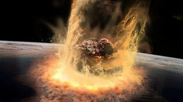
Comet impact on Earth are synonymous with great extinctions, but now research presented at the Goldschmidt geochemistry conference in Prague shows that early comet impact would have become a driving force to cause substantial synthesis of peptides — the first building blocks of life. This may have implications for the genesis of life on other worlds.
Dr Haruna Sugahara, from the Japan Agency for Marine-Earth Science and Technology (JAMSTEC) in Yokahama, and Dr Koichi Mimura, from Nagoya University performed a series of experiments to mimic the conditions of comet impacts on the Early Earth at the time when life first appeared, around 4 billion years ago.
They took frozen mixtures of amino acid, water ice and silicate (forsterite) at cryogenic condition (77 K), and used a propellant gun to simulate the shock of a comet impact. After analyzing the post-impact mixture with gas chromatography, they found that some of the amino acids had joined into short peptides of up to 3 units long (tripeptides).
Based on the experimental data, the researchers were able to estimate that the amount of peptides produced would be around the same as had been thought to be produced by normal terrestrial processes (such as lighting storms or hydration and dehydration cycles).
According to Haruna Sugahara: “Our experiment showed that the cold conditions of comets at the time of the impacts were key to this synthesis, as the type of peptide formed this way are more likely to evolve to longer peptides.
This finding indicates that comet impacts almost certainly played an important role in delivering the seeds of life to the early Earth. It also opens the likelihood that we will have seen similar chemical evolution in other extraterrestrial bodies, starting with cometary-derived peptides.
Within our own solar system the icy satellites of Jupiter and Saturn, such as Europa and Enceladus are likely to have undergone a similar comet bombardment. Indeed, the NASA stardust mission has shown the presence of the amino acid glycine in comets.
The production of short peptides is the key step in the chemical evolution of complex molecules. Once the process is kick-started, then much less energy is needed to make longer chain peptides in a terrestrial, aquatic environment.
Comet impacts are normally associated with mass extinction on Earth, but this works shows that they probably helped kick-start the whole process of life in the first place.”
Commenting, Professor Mark Burchell (University of Kent, UK) said: “This is a new piece of work which adds significantly to the exciting field of the origin of complex molecules on the Earth. It has long been known that ices under shock can generate and break bonds in complex organics. The detection of amino acids on comet 81P/Wild2 by the NASA Stardust mission in the last decade, and the now regular exciting news from the Rosetta mission to comet 67P/Churyumuv-Gerasimenko indicates that comets are a rich source of materials. Two key parts to this story are how complex molecules are initially generated on comets and then how they survive/evolve when the comet hits a planet like the Earth. Both of these steps can involve shocks which deliver energy to the icy body. For example, Zita Martins and colleagues recently showed how complex organic compounds can be synthesized on icy bodies via shocks. Now, building on earlier work, Dr Sughara and Dr Mimura have shown how amino acids on icy bodies can be turned into short peptide sequences, another key step along the path to life.”
Fluid-rich diamonds formed 200 km beneath Earth’s surface offer clues to how diamonds are made—and possibly how they can be found, according to new U of A research.
Some of the rich diamond deposits in the Northwest Territories may have been formed as a result of ancient seawater streaming into the deep roots of the continent, transported by plate tectonics, suggests new research from an international team of scientists in Canada, the U.S. and the U.K. The discovery further highlights the role played by plate tectonics in “recycling” surface materials into deep parts of the earth, building on the groundbreaking discovery by a University of Alberta team last year of vast quantities of water trapped more than 500 kilometres underground.
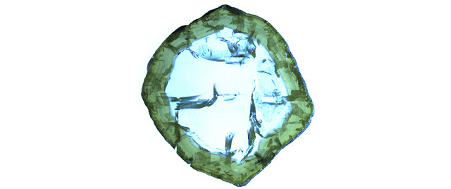
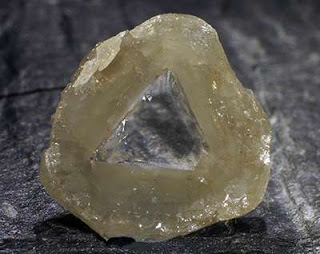
Diamond with a gem-quality core and fluid-rich “coat”. The coat contains millions of tiny fluid inclusions that trap pristine brine from 200 km depth. Credit: Anetta Banas
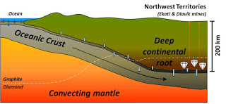
“With the ringwoodite discovery, we showed there is a lot of water trapped in really deep parts of the Earth, which probably all came from recycling ocean water,” explains Graham Pearson, professor in the U of A’s Department of Earth and Atmospheric Sciences and Canada Excellence Research Chair in Arctic Resources. “This new study really highlights that process—it clearly demonstrates that ocean water in this case has been subducted via an old oceanic slab into a slightly shallower but still very deep part of the Earth. From there it has pumped that brine into the bottom of the root beneath the Northwest Territories, and it’s made the diamonds.”
Ugly diamonds are a researcher’s best friend
The Northwest Territories is home to rich deposits of high-quality gem diamonds as well as so-called “low-quality” diamonds, which are covered in a coat of cloudy material. “They’re kind of ugly things,” laughs Pearson. “But all the most interesting diamonds are.”
All diamonds are formed from fluids, but only these less attractive coated stones still contain traces of their scientifically valuable source fluids. “[The fluids in the coats] are sky-high in sodium and potassium and chlorine, and it’s very difficult to get that stuff from the Earth’s normal mantle,” says Pearson. “It’s a big mystery—where does that come from? Well, we can show that maybe the most sensible place for it to come from is seawater, which is basically a sodium chloride solution.”
Pearson notes that this captive seawater likely became trapped in a massive slab of the Earth’s oceanic crust that was subducted beneath North America some hundreds of millions of years ago. The interaction of these seawater brines with the overlying mantle rocks produced a chemically diverse range of fluids from which diamonds crystallized, and could then be carried back to the Earth’s surface via an erupting host volcanic rock known as a kimberlite. These fluid-rich diamonds provide scientists with the most pristine examples of deep Earth fluids—from around 200 km beneath Earth’s surface.
“The beauty of the diamond is that because it’s such a robust capsule, it protects the material that it trapped at that depth from any subsequent change,” says Pearson. “It literally carries pristine bits of material from right where it came from, essentially unchanged.”
New facets of understanding
Schematic model of subduction of oceanic crust altered by seawater and the infiltration of brines into the base of the deep continental root beneath NWT, Canada, to make fluid-rich diamonds.
Although high-quality gem diamonds are normally estimated to have been formed three billion to 3.5 billion years ago, these poor-quality, fluid-rich diamonds appear to be just a few hundred million years old—significantly younger in the Earth’s geological timeline. One theory to explain this age difference is that the two types of diamonds are actually formed by similar processes, and then over time the fluid-rich stones transform into the gem diamonds. Pearson and his team plan to do further studies on the fluids found in these diamonds to test this model.
“What we appear to be finding more and more is that the standard model that used to be around—diamonds are only formed in very ancient times, 3.5 billion years ago, by a very specific process—is not true,” says Pearson. “There are more processes that form diamonds at a whole range of different times than we thought possible.”
Understanding more about how diamonds form can shape exploration models of how to find them, offering clues to help locate further deposits. Canada is the world’s third-highest diamond producer by value, and the majority of the product is retrieved from the Northwest Territories, where mining is a significant contributor to the province’s economy.
The findings of the study were published in Nature.
Reference:
“Highly saline fluids from a subducting slab as the source for fluid-rich diamonds.” Nature 524, 339–342 (20 August 2015) DOI: 10.1038/nature14857
In the D’Entrecasteaux Islands off Papua New Guinea, the rocks are giving rise to new ideas about the ways in which mountain chains form. A new scientific model inspired by data from the islands shows how the seemingly opposite processes of tectonic compression and extension can take place in the same region. It also shows how sections of earth’s crust that have been pushed deep under the surface can reverse course and rise in what in the geological time scale would be an instant. The model has implications for the understanding of how many mountain belts form.
The islands sit in the middle of an active, messy boundary between two major tectonic plates. Mountain belts like the Appalachians and the Alps formed in similar regions, where continental fragments, small ocean basins and island arcs smashed together.
In the last few decades, scientists have shown that rocks found in some mountain belts were formed at depths of 100 kilometers or more, where ultrahigh pressure minerals, like microdiamonds, form. It is accepted that continental rocks can get to that depth through subduction, when one plate is pushed under another.
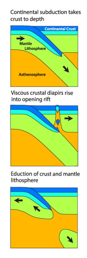
There is an ongoing debate over how these rocks rise to the surface. Some argue that small bits of subducted crust break off and pop up to the surface either as brittle slivers or flowing “diapirs” (see illustration). Others argue that an entire plate that has been subducted can reverse course and rise back up, a process known as eduction.
The new thermomechanical model, created by scientists at Lamont‐Doherty Earth Observatory and Aarhus University in Denmark, shows how both processes can occur together. It shows that the most deeply subducted crust can be warmed enough for pieces to break off and flow upward into diapirs. The diapirs only move up a short distance, so something else has to transport them to the surface. In this case, the model shows how it is the reversal in direction of motion of the subducted slab. The model also shows how reverse subduction can be triggered by the start of a new subduction zone nearby.
The model came out of an effort to understand new observations made in and around the D’Entracasteaux Islands, the only known place on earth where ultrahigh-pressure rocks are actively coming up. The new work is described in the early online version of the journal Geochemistry, Geophysics, Geosystems. The model shows that continental extension and the spreading of new ocean basin can occur after the subducted plate is pulled up. This scenario is consistent with Woodlark Basin, which is actively spreading to the east of the islands.
Lamont geophysicist Roger Buck points to Goodenough Basin, just south of the islands, as a possible test of the reverse subduction model. On geologic time scales, the basin appears to be very new. It has little sediment, 50 to 1,000 meters, compared to 5 to 10 kilometers of sediment in areas around it. “Essentially, the islands may be the tip of what was brought down and warmed up and became partially molten. If the ultrahigh-pressure rocks on the islands had to be 100 kilometers down to form, what do you do with the top 90 kilometers when it comes up? I think it was continental margin that came back up and flattened and is now the floor of the Goodenough Basin,” Buck said.
Buck and Kenni Dinesen Peterson of Aarhaus University used computer models to show how resistance to subducting buoyant continental crust can trigger initiation of a new subduction zone. In the case of Goodenough Basin, the new subduction zone is the New Britain Trench. The model suggests that the floor of Goodenough Basin rose up within the past 5 million years. It’s a premise that could be tested in the future by drilling into the basin’s floor. This may help us figure out why many mountain belts have such a complex array of structures and rocks formed at different depths.
Reference:
“Eduction, extension, and exhumation of ultrahigh-pressure rocks in metamorphic core complexes due to subduction initiation.” Geochem. Geophys. Geosyst., 16, DOI: 10.1002/2015GC005847
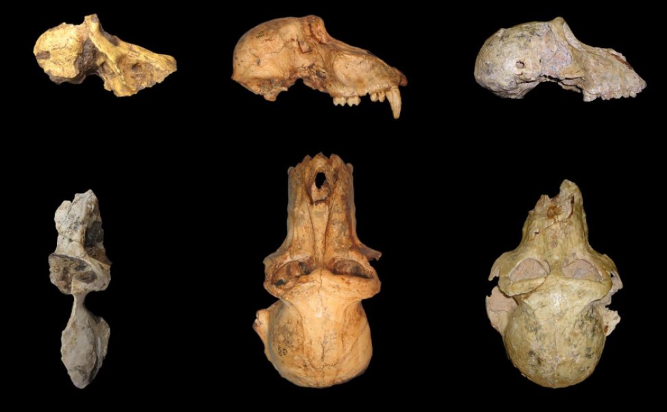
Here is a comparison of morphology in UW 88-886 (left), P. angusticepts males (CO 100, center), and P. izodi males (TP 89-11-1, right). Credit: Wits University
A team from Wits University’s Evolutionary Studies Institute has discovered a fossil monkey specimen representing the earliest baboon ever found.
Dating back more than 2 million years ago (between 2.026-2.36 million years ago), the partial skull was found at Malapa, in the Cradle of Humankind World Heritage Site, the same site where the partial skeletons of the new early hominin species, Australopithecus sediba, were discovered in 2010.
“Baboons are known to have co-existed with hominins at several fossil localities in East Africa and South Africa and they are sometimes even used as comparative models in human evolution,” says Dr Christopher Gilbert (Hunter College, CUNY), lead author of the study.
The skull, found during excavations for A. sediba, confirms earlier suggestions that the fossil baboon species to which it belongs, Papio angusticeps, was in fact closely related to modern baboons, and quite possibly the earliest known members of the modern baboon species Papio hamadryas.
Modern baboons (genus Papio) are typically divided into a number of populations recognised as either species or subspecies spread all throughout sub-Saharan Africa and into the Arabian Peninsula. Despite their evolutionary success, modern baboon origins in the fossil record have not well-understood or agreed upon.
“According to molecular clock studies, baboons are estimated to have diverged from their closest relatives by ~1.8 to 2.2 million years ago; however, until now, most fossil specimens known within this time range have been either too fragmentary to be definitive or too primitive to be confirmed as members of the living species Papio hamadryas,” says Gilbert.
“The specimen from Malapa and our current analyses help to confirm the suggestion of previous researchers that P. angusticeps may, in fact, be an early population of P. hamadryas.”
Analyses of the specimen at Malapa, and the group of fossil specimens traditionally placed in the fossil species P. angusticeps, suggest that P. angusticeps displays anatomy that is consistent with modern baboon populations.
“If you placed a number of P. angusticeps specimens into a modern osteology collection, I don’t think you’d be able pick them out as any different from those of modern baboons from East and South Africa,” says Gilbert.
Furthermore, the estimated age of the specimen from Malapa, ~2.026-2.36 Ma, is in almost perfect agreement with molecular clock analyses for the initial appearance of modern baboons. Thus, the specimen at Malapa may help to solve the evolutionary origins of these highly successful animals and confirm the estimates of molecular studies. In addition, because monkeys are widely recognised as key time-sensitive elements in the fossil record, the fact that the Malapa P. angusticeps specimen is well-dated allows future studies to better estimate the age of fossil sites where the species is found. South African early hominin sites, in particular, may be able to achieve more accurate age estimates on the basis of these new findings.
Reference:
Lee R. Berger et al. Papio Cranium from the Hominin-Bearing Site of Malapa: Implications for the Evolution of Modern Baboon Cranial Morphology and South African Plio-Pleistocene Biochronology. PLOS ONE, August 2015 DOI: 10.1371/journal.pone.0133361
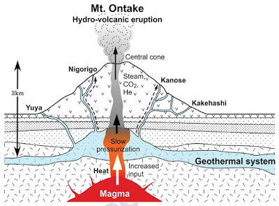
The increased input of magmatic volatiles is thought to have resulted in slow pressurization of the volcanic conduit leading to the event. Credit: Original figure was created by Michelle Laithier of University of Quebec at Montreal.
University of Tokyo researchers discovered an increase in a helium isotope during a ten-year period before the 2014 Mount Ontake eruption in central Japan. The finding suggests that this helium isotope anomaly is related to activation of the volcano’s magma system and could be a valuable marker for long-term risk mitigation concerning volcanic eruption.
Small quantities of the isotope helium-3 are present in the mantle, while helium-4 is produced in the crust and mantle by radioactive decay. A higher ratio of helium-3 to helium-4 therefore indicates that a sample of helium gas originates from the mantle rather than the crust. Previous research suggested that variation of helium isotopic ratios over time in crater fumaroles and hot springs correlates well with volcanic activity.
However, helium anomalies reported in these studies were all related to magmatic eruptions, and not to hydro-volcanic or phreatic eruptions, caused when a heat source such as magma vaporizes water to steam. Because phreatic eruptions are highly local phenomena, they are extremely difficult to predict. Mount Ontake, which erupted unexpectedly on September 27, 2014 just before noon, is believed to have been a phreatic eruption, and resulted in 58 deaths with 5 still missing.
An international research group lead by Professor Yuji Sano at the Atmosphere and Ocean Research Institute, the University of Tokyo, found that prior to the 2014 eruption, the helium-3 to helium-4 ratio at the hot spring closest to the volcanic cone increased significantly from June 2003 to November 2014, while that at distant hot springs showed no significant change. In addition, the helium isotopic ratios of the closest hot spring remained constant from November 1981 to June 2000.
These findings suggest that helium anomalies are also associated with phreatic eruptions. The research group suggests that increased input of magmatic gas over a ten-year period resulted in the slow pressurization of the volcanic conduit and eventually lead to the eruption.
“We were aware that helium isotopic ratios of the closest hot spring increased significantly from June 2003 to July 2009. At that time we did not understand the reason behind it,” recalls Sano. He adds, “Our findings suggest that the anomaly was related to the 2014 eruption and may have been a precursor. Although this new research does not offer a way to predict an eruption in the short-term, it offers a guide that may be useful for long-term risk management and disaster mitigation.”
Reference:
Yuji Sano, Takanori Kagoshima, Naoto Takahata, Yoshiro Nishio, Emilie Roulleau, Daniele L. Pinti, Tobias P. Fischer. Ten-year helium anomaly prior to the 2014 Mt Ontake eruption. Scientific Reports, 2015; 5: 13069 DOI: 10.1038/srep13069
Note: The above post is reprinted from materials provided by University of Tokyo.
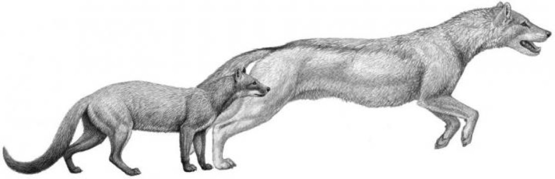
Two early dogs, Hesperocyon, left and the later Sunkahetanka, were both ambush-style predators. As climate changes transformed their habitat, dogs evolved pursuit hunting styles and forelimb anatomy to match. Credit: Mauricio Anton
Old dogs can teach humans new things about evolution. In Nature Communications a new study of North American dog fossils as old as 40 million years suggests that the evolutionary path of whole groups of predators can be a direct consequence of climate change.
“It’s reinforcing the idea that predators may be as directly sensitive to climate and habitat as herbivores,” said Christine Janis, professor of ecology and evolutionary biology at Brown University, who worked with lead author Borja Figueirido, a former Brown Fulbright postdoctoral researcher who is now a professor at the Universidad de Málaga in Spain. “Although this seems logical, it hadn’t been demonstrated before.”
The climate in North America’s heartland back around 40 million years ago was warm and wooded. Dogs are native to North America. The species of the time, fossils show, were small animals that would have looked more like mongooses than any dogs alive today and were well-adapted to that habitat. Their forelimbs were not specialized for running, retaining the flexibility to grapple with whatever meal unwittingly walked by.
But beginning just a few million years later, the global climate began cooling considerably and in North America the Rocky Mountains had reached a threshold of growth that made the continental interior much drier. The forests slowly gave way to open grasslands.
Pups of the plains
Did this transition affect the evolution of carnivores? To find out, Figueirido and the research team, including Jack Tseng of the American Museum of Natural History in New York, examined the elbows and teeth of 32 species of dogs spanning the period from ca. 40 million years ago to 2 million years ago. They saw clear patterns in those bones at the museum: At the same time that climate change was opening up the vegetation, dogs were evolving from ambushers to pursuit-pounce predators like modern coyotes or foxes — and ultimately to those dogged, follow-a-caribou-for-a-whole-day pursuers like wolves in the high latitudes.
“The elbow is a really good proxy for what carnivores are doing with their forelimbs, which tells their entire locomotion repertoire,” Janis said.
The telltale change in those elbows has to do with the structure of the base where the humerus articulates with the forearm, changing from one where the front paws could swivel (palms can be inward or down) for grabbing and wrestling prey to one with an always downward-facing structure specialized for endurance running. Modern cats still rely on ambush rather than the chase (cheetahs are the exception) and have the forelimbs to match, Janis said, but canines signed up for lengthier pursuits.
In addition, the dogs’ teeth trended toward greater durability, Figueirido’s team found, consistent perhaps with the need to chow down on prey that had been rolled around in the grit of the savannah, rather than a damp, leafy forest floor.
Not an ‘arms race’ of limbs
The study, with some of Janis’ prior research, suggests that predators do not merely evolve as an “arms race” response to their prey. They don’t develop forelimbs for speedy running just because the deer and the antelope run faster. While the herbivores of this time were evolving longer legs, the predator evolution evident in this study tracked in time directly with the climate-related changes to habitat rather than to the anatomy of their prey species.
After all, it wasn’t advantageous to operate as a pursuit-and-pounce predator until there was room to run.
“There’s no point in doing a dash and a pounce in a forest,” Janis quipped. “They’ll smack into a tree.”
If predators evolved with climate change over the last 40 million years, the authors argue, then they likely will have to continue in response to the human-created climate change underway now. The new results could help predict the effects we are setting in motion.
“Now we’re looking into the future at anthropogenic changes,” Janis said.
Reference:
B. Figueirido, A. Martín-Serra, Z. J. Tseng, C. M. Janis. Habitat changes and changing predatory habits in North American fossil canids. Nature Communications, 2015; 6: 7976 DOI: 10.1038/ncomms8976
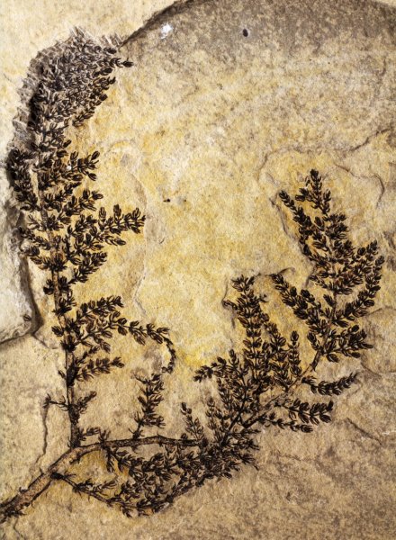
This is a large intact specimen of the fossil, Montsechia. Usually only small fragmentary pieces of the fossil are found. Credit: David Dilcher
Indiana University paleobotanist David Dilcher and colleagues in Europe have identified a 125 million- to 130 million-year-old freshwater plant as one of earliest flowering plants on Earth.
The finding, reported Aug. 17 in the Proceedings of the National Academy of Sciences, represents a major change in the presumed form of one of the planet’s earliest flowers, known as angiosperms.
“This discovery raises significant questions about the early evolutionary history of flowering plants, as well as the role of these plants in the evolution of other plant and animal life,” said Dilcher, an emeritus professor in the IU Bloomington College of Arts and Sciences’ Department of Geological Sciences.
The aquatic plant, Montsechia vidalii, once grew abundantly in freshwater lakes in what are now mountainous regions in Spain. Fossils of the plant were first discovered more than 100 years ago in the limestone deposits of the Iberian Range in central Spain and in the Montsec Range of the Pyrenees, near the country’s border with France.
Also previously proposed as one of the earliest flowers is Archaefructus sinensis, an aquatic plant found in China.
“A ‘first flower’ is technically a myth, like the ‘first human,'” said Dilcher, an internationally recognized expert on angiosperm anatomy and morphology who has studied the rise and spread of flowering plants for decades. “But based on this new analysis, we know now that Montsechia is contemporaneous, if not more ancient, than Archaefructus.”
He also asserted that the fossils used in the study were “poorly understood and even misinterpreted” during previous analyses.
“The reinterpretation of these fossils provides a fascinating new perspective on a major mystery in plant biology,” said Donald H. Les, a professor of ecology and evolutionary biology at the University of Connecticut, who is the author of a commentary on the discovery in the journal PNAS. “David’s work is truly an important contribution to the continued quest to unravel the evolutionary and ecological events that accompanied the rise of flowering plants to global prominence.”
The conclusions are based upon careful analyses of more than 1,000 fossilized remains of Montsechia, whose stems and leaf structures were coaxed from stone by applying hydrochloric acid on a drop-by-drop basis. The plant’s cuticles — the protective film covering the leaves that reveals their shape — were also carefully bleached using a mixture of nitric acid and potassium chlorate.
Examination of the specimens was conducted under a stereomicroscope, light microscope and scanning electron microscope.
The age of the plant at 125 million to 130 million years is based upon comparisons to other fossils in the same area, notably the freshwater algae charophytes, which places Montsechia in the Barremian age of the early Cretaceous period, making this flowering plant a contemporary of dinosaurs such as the brachiosaurus and iguanodon.
The precise, painstaking analysis of fossilized structures remains crucial to paleobotany, in contrast to other biological fields, due to the current inability to know the molecular characters of ancient plants from millions of years ago, Dilcher said.
This careful examination was particularly important to Montsechia since most modern observers might not even recognize the fossil as a flowering plant.
“Montsechia possesses no obvious ‘flower parts,’ such as petals or nectar-producing structures for attracting insects, and lives out its entire life cycle under water,” he said. “The fruit contains a single seed” — the defining characteristic of an angiosperm — “which is borne upside down.”
In terms of appearance, Dilcher said, Montsechia resembles its most modern descendent, identified in the study as Ceratophyllum. Also known as coontails or hornworts, Ceratophyllum is a dark green aquatic plant whose coarse, tufty leaves make it a popular decoration in modern aquariums and koi ponds.
Next up, Dilcher and colleagues want to understand more about the species connecting Montsechia and Ceratophyllum, as well as delve deeper into when precisely other species of angiosperms branched off from their ancient forefathers.
“There’s still much to be discovered about how a few early species of seed-bearing plants eventually gave rise to the enormous, and beautiful, variety of flowers that now populate nearly every environment on Earth,” he said.
Reference:
David L. Dilcherd et al. Montsechia, an ancient aquatic angiosperm. PNAS, August 2015 DOI: 10.1073/pnas.1509241112
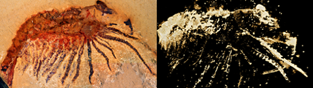
The figure on the right shows a light micrograph of the fossil, while the microtomographic image left reveals fine details of structures hitherto concealed within the slab.
Ludwig Maximilian University researchers have used computed microtomography (micro-CT) to identify to the species level an exceptionally wellpreserved fossil arthropod from the famous Chengjiang Lagerstätte in China.
Modern imaging methods make it possible to perform detailed, non-invasive studies on the internal structures of irreplaceable fossil specimens. Researchers led by Dr. Yu Liu of LMU’s Department of Biology II now demonstrate the power of this approach by using computed microtomography (micro-CT) to investigate a specimen recovered from the famous fossil beds of Chengjiang in southwestern China. The results of the study, which appear in the online Open Access journal Scientific Reports, demonstrate the ability of micro-CT to reveal anatomical details preserved inside fossil slabs.
The fossil Lagerstätte Chengjiang in China is a UNESCO World Heritage Site, which harbors a rich fossil assemblage dating from 520 million years ago. The rocks preserved here are among the oldest that document the so-called Cambrian explosion – the relatively abrupt appearance of a highly diverse, species-rich multicellular fauna in the fossil record. And many of the specimens discovered in these beds are extremely well preserved. In particular, their soft parts have left clear impressions in the sediments that accumulated here. Imprints of organisms with mineralized skeletons often extend for several millimeters below the surface of the slabs of sediment in which they are embedded. In order to study their structure, such specimens must first be removed from the surrounding rock matrix. “Because this inevitably involves the destruction of at least some of their fine structure, most of the published work on Chengjiang’s fossils is based on careful examination of surface structures with the help of optical and fluorescence microscopy,” as Yu Liu explains.
The LMU team now reports the first in-depth microtomographic study of a three-dimensionally preserved fossil from Chengjiang. The term micro-CT refers to a method in which multiple X-radiographs of a specimen are taken from different angles, and then assembled with the help of mathematical procedures to yield a three-dimensional model of the original. It is now a well-established analytical tool in palaeontology, but has not yet been widely applied to fossils from Chengjiang. Yu Liu’s study uncovers internal structures in a specimen recovered from the site, which allow the fossil to be identified as Xandarella spectaculum, a rare species of arthropod that shows similarities to the iconic (but now extinct) trilobites, and is known only from Chengjiang. The three-dimensional reconstruction reveals informative details of the fossil’s morphology, which had hitherto remained hidden in the rock matrix. On the basis of the new results, Yu Liu confidently asserts that “microtomography is a powerful technique for the analysis of the three-dimensionally preserved specimens recovered at Chengjiang.”
Reference:
“When a 520 million-year-old Chengjiang fossil meets a modern micro-CT – a case study.” Scientific Reports 5, (2015) DOI: 10.1038/srep12802
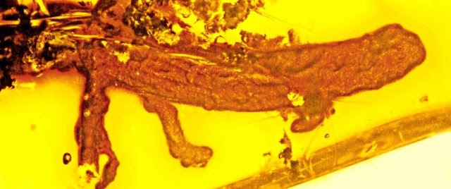
This is the first-ever discovery of a salamander preserved in amber, from an unlikely spot — the Dominican Republic, where all salamanders are now extinct. Credit: Photo by George Poinar, Jr., courtesy of Oregon State University
More than 20 million years ago, a short struggle took place in what is now the Dominican Republic, resulting in one animal getting its leg bitten off by a predator just before it escaped. But in the confusion, it fell into a gooey resin deposit, to be fossilized and entombed forever in amber.
The fossil record of that event has revealed something not known before — that salamanders once lived on an island in the Caribbean Sea. Today, they are nowhere to be found in the entire Caribbean area.
The never-before-seen and now extinct species of salamander, named Palaeoplethodon hispaniolae by the authors of the paper, adds more clues to the ecological and geological history of the islands of the Caribbean. Findings about its brief life and traumatic end — it was just a baby — have been published in the journal Palaeodiversity, by researchers from Oregon State University and the University of California at Berkeley.
“I was shocked when I first saw it in amber,” said George Poinar, Jr., a professor emeritus in the OSU College of Science, and a world expert in the study of insects, plants and other life forms preserved in amber, all of which allow researchers to reconstruct the ecology of ancient ecosystems.
“There are very few salamander fossils of any type, and no one has ever found a salamander preserved in amber,” Poinar said. “And finding it in Dominican amber was especially unexpected, because today no salamanders, even living ones, have ever been found in that region.”
This fossil salamander belonged to the family Plethodontidae, a widespread family that today is still very common in North America, particularly the Appalachian Mountains. But it had back and front legs lacking distinct toes, just almost complete webbing with little bumps on them. As such, it might not have been as prolific a climber as some modern species, Poinar said, and it probably lived in small trees or tropical flowering plants.
This specimen, Poinar said, came from an amber mine in the northern mountain range of the Dominican Republic, between Puerto Plata and Santiago.
“The discovery of this fossil shows there once were salamanders in the Caribbean, but it’s still a mystery why they all went extinct,” Poinar said. “They may have been killed by some climatic event, or were vulnerable to some type of predator.”
Also a mystery, he said, is how salamanders got there to begin with. The physical evidence suggests the fossil represents an early lineage of phethodon salamanders that evolved in tropical America.
This fossil is 20-30 million years old, and its lineage may go back 40-60 million years ago when the Proto-Greater Antilles, that now include islands such as Cuba, Jamaica, Puerto Rico and Hispaniola, were still joined to North and South America. Salamanders may have simply stayed on the islands as they began their tectonic drift across the Caribbean Sea. They also may have crossed a land bridge during periods of low sea level, or it’s possible a few specimens could have floated in on debris, riding a log across the ocean.
Such findings, Poinar said, help both ecologists and geologists to reconstruct ancient events of Earth’s history.
“There have been fossils of rhinoceroses found in Jamaica, jaguars in the Dominican Republic, and the tree that produced the Dominican amber fossils is most closely related to one that’s native to East Africa,” Poinar said. “All of these findings help us reconstruct biological and geological aspects of ancient ecosystems.”
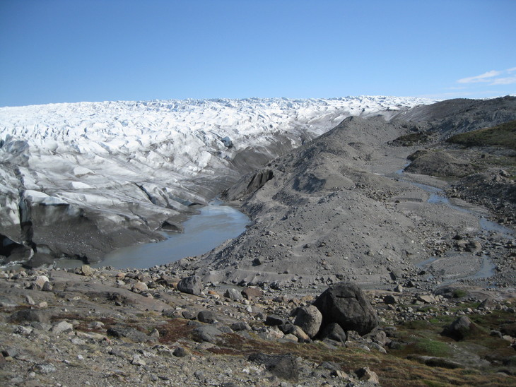
The margin of the Greenland Ice Sheet in summer 2011. Credit: Patrick Applegate
Albedo modification, an emerging technology with the potential to offset some aspects of climate change, shouldn’t be counted on as a short-term solution to stop rising global sea levels, according to a new study from Penn State geoscientists.
“In the short term, the first few decades to the first century after you start doing albedo modification, it’s not as effective in avoiding sea-level rise from the Greenland Ice Sheet as you might think,” said Patrick Applegate, a research associate in Penn State’s Earth and Environmental Systems Institute. “The rate of sea-level rise goes down, but sea-level rise from the ice sheet doesn’t stop.”
Researchers used computer model experiments to test how the Greenland Ice Sheet would react to albedo modification, also called solar radiation management geoengineering, a proposed technology to cool down the Earth’s temperature by reflecting some sunlight away from the planet. They found the ice sheet might contribute to sea-level rise for decades to centuries after albedo modification began.
The findings, published this week in the journal Environmental Research Letters, provide a nuanced picture of how albedo modification might affect future sea-level rise, and build on a previous study that looked at the effect of albedo modification on the Greenland Ice Sheet over a much longer period of time.
“There has been one other study that used broadly similar methods, but they looked at really long timescales,” Applegate said. “Many people are also interested in what happens over the next few decades or centuries, so we zoomed in on shorter time scales for our study. And there you get a very different answer.”
The researchers looked at a three-dimensional ice sheet model that included some important feedbacks.
One such feedback is the size of the ice sheet itself. The Greenland Ice Sheet is like a tall, white mountain. Its height means it’s much colder at the top of the ice sheet than at sea level. If the ice sheet has already partly melted when albedo modification begins, the cold area at the top might be smaller, making it harder to save the ice sheet by reducing temperatures.
The Greenland Ice Sheet contains enough ice to raise global sea level by about 24 feet if the sheet were to melt entirely. If that were to happen, many people who live near present-day sea level would be at risk of being displaced by flooding.
“Albedo modification is not something that can be done locally. That means the world community has to make some kind of analysis of the costs versus the benefits of albedo modification,” Applegate said. “We argue that the benefits may be smaller than we thought.”
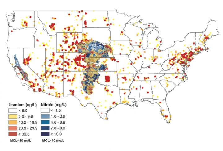
The intensity of groundwater contamination via uranium (red) and nitrate (blue) is shown in two major aquifers and other sites through out the nation. UNL researcher Karrie Weber says the availability of uranium data pales compared to that of nitrate. Credit: University of Nebraska-Lincoln
Nearly 2 million people throughout the Great Plains and California above aquifer sites contaminated with natural uranium that is mobilized by human-contributed nitrate, according to a study from the University of Nebraska-Lincoln.
Data from roughly 275,000 groundwater samples in the High Plains and Central Valley aquifers show that many Americans live less than two-thirds of a mile from wells that often far exceed the uranium guideline set by the Environmental Protection Agency.
The study reports that 78 percent of the uranium-contaminated sites were linked to the presence of nitrate, a common groundwater contaminant that originates mainly from chemical fertilizers and animal waste. Nitrate mobilizes naturally occurring uranium through a series of bacterial and chemical reactions that oxidize the radioactive mineral, making it soluble in groundwater.
UNL researchers Karrie Weber and Jason Nolan found that the High Plains aquifer contains uranium concentrations up to 89 times the EPA standard and nitrate concentrations up to 189 times greater. The uranium and nitrate levels of the California-based Central Valley aquifer measured up to 180 and 34 times their respective EPA thresholds.
The authors published their findings in the August edition of the journal Environmental Science and Technology Letters. Their research was funded in part by the U.S. Geological Survey.
“It needs to be recognized that uranium is a widespread contaminant,” said Weber, assistant professor of biological, Earth and atmospheric sciences. “And we are creating this problem by producing a primary contaminant that leads to a secondary one.”
Prior research has suggested that prolonged drinking of uranium-contaminated water may lead, or make people more susceptible, to kidney damage and elevated blood pressure. According to Weber, peer-reviewed studies have also indicated that food crops can accumulate uranium when irrigated by water containing high concentrations of it.
The High Plains aquifer — the largest in the United States — provides drinking water and irrigation for an eight-state swath that stretches from South Dakota through Nebraska and into northern Texas. As California’s largest reservoir, the Central Valley aquifer sits beneath some of the state’s most fertile agricultural land. According to a 2012 census from the U.S. Department of Agriculture, the two aquifers irrigate cropland that accounts for one-sixth of the annual revenue generated by U.S. agriculture.
The researchers also determined that only one of the six wells located near a former or current mining site was contaminated. This finding counters the notion that uranium contamination stems primarily from mining operations or spent nuclear fuel, Weber said.
“We hope that this study serves as a catalyst to get other people interested in this issue,” she said. “If the problem is this widespread, more research needs to be done. We’re limited by the data that’s been collected, and uranium isn’t often monitored.”
Weber said the expense of water treatment plants — specialized facilities that can cost tens of millions of dollars — often puts them out of financial reach for smaller and rural communities. Addressing the issue might require managing groundwater and focusing on the aquifers’ sediment, which houses bacteria that can help control uranium by breathing and eating it, she said.
Regardless of the approach, Weber said it is important for decision-makers and researchers to account for the presence of uranium in U.S. water sources.
“When you start thinking about how much water is drawn from these aquifers, it’s substantial relative to anywhere else in the world,” Weber said. “These two aquifers are economically important — they play a significant role in feeding the nation — but they’re also important for health.
“What’s the point of having water if you can’t drink it or use it for irrigation?”
Note: The above post is reprinted from materials provided by University of Nebraska-Lincoln. The original article was written by Scott Schrage, University Communications.