The Eocene epoch, lasting from 56 to 33.9 million years ago, is a major division of the geologic timescale and the second epoch of the Paleogene Period in the Cenozoic Era. The Eocene spans the time from the end of the Palaeocene Epoch to the beginning of the Oligocene Epoch. The start of the Eocene is marked by a brief period in which the concentration of the carbon isotope 13C in the atmosphere was exceptionally low in comparison with the more common isotope 12C. The end is set at a major extinction event called the Grande Coupure (the “Great Break” in continuity) or the Eocene–Oligocene extinction event, which may be related to the impact of one or more large bolides in Siberia and in what is now Chesapeake Bay. As with other geologic periods, the strata that define the start and end of the epoch are well identified, though their exact dates are slightly uncertain.
The name Eocene comes from the Greek ἠώς (eos, dawn) and καινός (kainos, new) and refers to the “dawn” of modern (‘new’) fauna that appeared during the epoch.
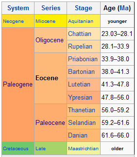
Subdivisions
The Eocene epoch is usually broken into Early and Late, or—more usually—Early, Middle, and Late subdivisions. The corresponding rocks are referred to as Lower, Middle, and Upper Eocene. Of the stages shown above, the Ypresian and occasionally the Lutetian constitute the Early, the Priabonian and sometimes the Bartonian the Late state; alternatively, the Lutetian and Bartonian are united as the Middle Eocene.
Climate
The Eocene Epoch contained a wide variety of different climate conditions that includes the warmest climate in the Cenozoic Era and ends in an icehouse climate. The evolution of the Eocene climate began with warming after the end of the Palaeocene-Eocene Thermal Maximum (PETM) at 56 million years ago to a maximum during the Eocene Optimum at around 49 million years ago. During this period of time, little to no ice was present on Earth with a smaller difference in temperature from the equator to the poles. Following the maximum was a descent into an icehouse climate from the Eocene Optimum to the Eocene-Oligocene transition at 34 million years ago. During this decrease ice began to reappear at the poles, and the Eocene-Oligocene transition is the period of time where the Antarctic ice sheet began to rapidly expand.
Atmospheric greenhouse gas evolution
Greenhouse gases, in particular carbon dioxide and methane, played a significant role during the Eocene in controlling the surface temperature. The end of the PETM was met with a very large sequestration of carbon dioxide in the form of methane clathrate, coal, and crude oil at the bottom of the Arctic Ocean, that reduced the atmospheric carbon dioxide. This event was similar in magnitude to the massive release of greenhouse gasses at the beginning of the PETM, and it is hypothesized that the sequestration was mainly due to organic carbon burial and weathering of silicates. For the early Eocene there is much discussion on how much carbon dioxide is in the atmosphere. This is due to numerous proxies representing different atmospheric carbon dioxide content. For example, diverse geochemical and paleontological proxies indicate that at the maximum of global warmth the atmospheric carbon dioxide values were at 700 – 900 ppm while other proxies such as pedogenic (soil building) carbonate and marine boron isotopes indicate large changes of carbon dioxide of over 2,000 ppm over periods of time of less than 1 million years. Sources for this large influx of carbon dioxide could be attributed to volcanic out-gassing due to North Atlantic rifting or oxidation of methane stored in large reservoirs deposited from the PETM event in the sea floor or wetland environments. For contrast, today the carbon dioxide levels are at 400 ppm or .04%.
During the early Eocene, methane was another greenhouse gas that had a drastic effect on the climate. In comparison to carbon dioxide, methane has much higher consequences with regards to temperature as methane has ~23 times more effect per molecule than carbon dioxide on a 100-year scale (it has a higher global warming potential). The majority of the methane released to the atmosphere during this period of time would have been from wetlands, swamps, and forests. The atmospheric methane concentration today is 0.000179% or 1.79 ppmv. Due to the warmer climate and sea level rise associated with the early Eocene, more wetlands, more forests, and more coal deposits would be available for methane release. Comparing the early Eocene production of methane to current levels of atmospheric methane, the early Eocene would be able to produce triple the amount of current methane production. The warm temperatures during the early Eocene could have increased methane production rates, and methane that is released into the atmosphere would in turn warm the troposphere, cool the stratosphere, and produce water vapor and carbon dioxide through oxidation. Biogenic production of methane produces carbon dioxide and water vapor along with the methane, as well as yielding infrared radiation. The breakdown of methane in an oxygen atmosphere produces carbon monoxide, water vapor and infrared radiation. The carbon monoxide is not stable so it eventually becomes carbon dioxide and in doing so releases yet more infrared radiation. Water vapor, traps more infrared than does carbon dioxide.
The middle to late Eocene marks not only the switch from warming to cooling, but also the change in carbon dioxide from increasing to decreasing. At the end of the Eocene Optimum, carbon dioxide began decreasing due to increased siliceous plankton productivity and marine carbon burial. At the beginning of the middle Eocene an event that may have triggered or helped with the draw down of carbon dioxide was the Azolla event at around 49 million years ago. With the equable climate during the early Eocene, warm temperatures in the arctic allowed for the growth of azolla, which is a floating aquatic fern, on the Arctic Ocean. Compared to current carbon dioxide levels, these azolla grew rapidly in the enhanced carbon dioxide levels found in the early Eocene. As these azolla sank into the Arctic Ocean, they became buried and sequestered their carbon into the seabed. This event could have led to a draw down of atmospheric carbon dioxide of up to 470 ppm. Assuming the carbon dioxide concentrations were at 900 ppmv prior to the Azolla Event they would have dropped to 430 ppmv, or 40 ppmv more than they are today, after the Azolla Event. Another event during the middle Eocene that was a sudden and temporary reversal of the cooling conditions was the Middle Eocene Climatic Optimum. At around 41.5 million years ago, stable isotopic analysis of samples from Southern Ocean drilling sites indicated a warming event for 600 thousand years. A sharp increase in atmospheric carbon dioxide was observed with a maximum of 4000 ppm: the highest amount of atmospheric carbon dioxide detected during the Eocene. The main hypothesis for such a radical transition was due to the continental drift and collision of the India continent with the Asia continent and the resulting formation of the Himalayas. Another hypothesis involves extensive sea floor rifting and metamorphic decarbonation reactions releasing considerable amounts of carbon dioxide to the atmosphere.
At the end of the Middle Eocene Climatic Optimum, cooling and the carbon dioxide drawdown continued through the late Eocene and into the Eocene-Oligocene transition around 34 million years ago. Multiple proxies, such as oxygen isotopes and alkenones, indicate that at the Eocene-Oligocene transition, the atmospheric carbon dioxide concentration had decreased to around 750-800 ppm, approximately twice that of present levels.
Early Eocene and the equable climate problem
One of the unique features of the Eocene’s climate as mentioned before was the equable and homogeneous climate that existed in the early parts of the Eocene. A multitude of proxies support the presence of a warmer equable climate being present during this period of time. A few of these proxies include the presence of fossils native to warm climates, such as crocodiles, located in the higher latitudes, the presence in the high-latitudes of frost-intolerant flora such as palm trees which cannot survive during sustained freezes, and fossils of snakes found in the tropics that would require much higher average temperatures to sustain them. Using isotope proxies to determine ocean temperatures indicate sea surface temperatures in the tropics as high as 35 °C (95 °F) and bottom water temperatures that are 10 °C (18 °F) higher than present day values. With these bottom water temperatures, temperatures in areas where deep-water forms near the poles are unable to be much cooler than the bottom water temperatures.
An issue arises, however, when trying to model the Eocene and reproduce the results that are found with the proxy data. Using all different ranges of greenhouse gasses that occurred during the early Eocene, models were unable to produce the warming that was found at the poles and the reduced seasonality that occurs with winters at the poles being substantially warmer. The models, while accurately predicting the tropics, tend to produce significantly cooler temperatures of up to 20 °C (36 °F) underneath the actual determined temperature at the poles. This error has been classified as the “equable climate problem”. To solve this problem, the solution would involve finding a process to warm the poles without warming the tropics. Some hypotheses and tests which attempt to find the process are listed below.
Large lakes
Due to the nature of water as opposed to land, less temperature variability would be present if a large body of water is also present. In an attempt to try to mitigate the cooling polar temperatures, large lakes were proposed to mitigate seasonal climate changes. To replicate this case, a lake was inserted into North America and a climate model was run using varying carbon dioxide levels. The model runs concluded that while the lake did reduce the seasonality of the region greater than just an increase in carbon dioxide, the addition of a large lake was unable to reduce the seasonality to the levels shown by the floral and faunal data.
Ocean heat transport
The transport of heat from the tropics to the poles, much like how ocean heat transport functions in modern times, was considered a possibility for the increased temperature and reduced seasonality for the poles. With the increased sea surface temperatures and the increased temperature of the deep ocean water during the early Eocene, one common hypothesis was that due to these increases there would be a greater transport of heat from the tropics to the poles. Simulating these differences, the models produced lower heat transport due to the lower temperature gradients and were unsuccessful in producing an equable climate from only ocean heat transport.
Orbital parameters
While typically seen as a control on ice growth and seasonality, the orbital parameters were theorized as a possible control on continental temperatures and seasonality. Simulating the Eocene by using an ice free planet, eccentricity, obliquity, and precession were modified in different model runs to determine all the possible different scenarios that could occur and their effects on temperature. One particular case led to warmer winters and cooler summer by up to 30% in the North American continent, and it reduced the seasonal variation of temperature by up to 75%. While orbital parameters did not produce the warming at the poles, the parameters did show a great effect on seasonality and needed to be considered.
Polar stratospheric clouds
Another method considered for producing the warm polar temperatures were polar stratospheric clouds. Polar stratospheric clouds are clouds that occur in the lower stratosphere at very low temperatures. Polar stratospheric clouds have a great impact on radiative forcing. Due to their minimal albedo properties and their optical thickness, polar stratospheric clouds act similar to a greenhouse gas and traps outgoing longwave radiation. Different types of polar stratospheric clouds occur in the atmosphere: polar stratospheric clouds that are created due to interactions with nitric or sulfuric acid and water (Type I) or polar stratospheric clouds that are created with only water ice (Type II).
Methane is an important factor in the creation of the primary Type II polar stratospheric clouds that were created in the early Eocene. Since water vapor is the only supporting substance used in Type II polar stratospheric clouds, the presence of water vapor in the lower stratosphere is necessary where in most situations the presence of water vapor in the lower stratosphere is rare. When methane is oxidized, a significant amount of water vapor is released. Another requirement for polar stratospheric clouds is cold temperatures to ensure condensation and cloud production. Polar stratospheric cloud production, since it requires the cold temperatures, is usually limited to nighttime and winter conditions. With this combination of wetter and colder conditions in the lower stratosphere, polar stratospheric clouds could have formed over wide areas in Polar Regions.
To test the polar stratospheric clouds effects on the Eocene climate, models were run comparing the effects of polar stratospheric clouds at the poles to an increase in atmospheric carbon dioxide.The polar stratospheric clouds had a warming effect on the poles, increasing temperatures by up to 20 °C in the winter months. A multitude of feedbacks also occurred in the models due to the polar stratospheric clouds’ presence. Any ice growth was slowed immensely and would lead to any present ice melting. Only the poles were affected with the change in temperature and the tropics were unaffected, which with an increase in atmospheric carbon dioxide would also cause the tropics to increase in temperature. Due to the warming of the troposphere from the increased greenhouse effect of the polar stratospheric clouds, the stratosphere would cool and would potentially increase the amount of polar stratospheric clouds.
While the polar stratospheric clouds could explain the reduction of the equator to pole temperature gradient and the increased temperatures at the poles during the early Eocene, there are a few drawbacks to maintaining polar stratospheric clouds for an extended period of time. Separate model runs were used to determine the sustainability of the polar stratospheric clouds. Methane would need to be continually released and sustained to maintain the lower stratospheric water vapor. Increasing amounts of ice and condensation nuclei would be need to be high for the polar stratospheric cloud to sustain itself and eventually expand.
Hyperthermals through the Early Eocene
During the warming in the Early Eocene between 52 and 55 million years ago, there were a series of short-term changes of carbon isotope composition in the ocean. These isotope changes occurred due to the release of carbon from the ocean into the atmosphere that led to a temperature increase of 4-8 °C (7.2-14.4 °F) at the surface of the ocean. These hyperthermals led to increased perturbations in planktonic and benthic foraminifera, with a higher rate of sedimentation as a consequence of the warmer temperatures. Recent analysis of and research into these hyperthermals in the early Eocene has led to hypotheses that the hyperthermals are based on orbital parameters, in particular eccentricity and obliquity. The hyperthermals in the early Eocene, notably the Palaeocene-Eocene Thermal Maximum (PETM), the Eocene Thermal Maximum 2 (ETM2), and the Eocene Thermal Maximum 3 (ETM3), were analyzed and found that orbital control may have had a role in triggering the ETM2 and ETM3.
Greenhouse to icehouse climate
The Eocene is not only known for containing the warmest period during the Cenozoic, but it also marked the decline into an icehouse climate and the rapid expansion of the Antarctic ice sheet. The transition from a warming climate into a cooling climate began at ~49 million years ago. Isotopes of carbon and oxygen indicate a shift to a global cooling climate. The cause of the cooling has been attributed to a significant decrease of >2000 ppm in atmospheric carbon dioxide concentrations. One proposed cause of the reduction in carbon dioxide during the warming to cooling transition was the Azolla event. The increased warmth at the poles, the isolated Arctic basin during the early Eocene, and the significantly high amounts of carbon dioxide possibly led to azolla blooms across the Arctic Ocean. The isolation of the Arctic Ocean led to stagnant waters and as the azolla sank to the sea floor, they became part of the sediments and effectively sequestered the carbon. The ability for the azolla to sequester carbon is exceptional, and the enhanced burial of azolla could have had a significant effect on the world atmospheric carbon content and may have been the event to begin the transition into an ice house climate. Cooling after this event continued due to continual decrease in atmospheric carbon dioxide from organic productivity and weathering from mountain building.
Global cooling continued until there was a major reversal from cooling to warming indicated in the Southern Ocean at around 42-41 million years ago. Oxygen isotope analysis showed a large negative change in the proportion of heavier oxygen isotopes to lighter oxygen isotopes, which indicates an increase in global temperatures. This warming event is known as the Middle Eocene Climatic Optimum. The cause of the warming is considered to primarily be due to carbon dioxide increases, since carbon isotope signatures rule out major methane release during this short term warming. The increase in atmospheric carbon dioxide is considered to be due to increased seafloor spreading rates between Australia and Antarctica and increased amounts of volcanism in the region. Another possible atmospheric carbon dioxide increase could be during a sudden increase with metamorphic release during the Himalayan orogeny, however data on the exact timing of metamorphic release of atmospheric carbon dioxide is not well resolved in the data. Recent studies have mentioned, however, that the removal of the ocean between Asia and India could release significant amounts of carbon dioxide.This warming is short lived, as benthic oxygen isotope records indicate a return to cooling at ~40 million years ago.
Cooling continued throughout the rest of the Late Eocene into the Eocene-Oligocene transition. During the cooling period, benthic oxygen isotopes show the possibility of ice creation and ice increase during this later cooling. The end of the Eocene and beginning of the Oligocene is marked with the massive expansion of area of the Antarctic ice sheet that was a major step into the icehouse climate. Along with the decrease of atmospheric carbon dioxide reducing the global temperature, orbital factors in ice creation can be seen with 100,000 year and 400,000 year fluctuations in benthic oxygen isotope records. Another major contribution to the expansion of the ice sheet was the creation of the Antarctic circumpolar current. The creation of the Antarctic circumpolar current would isolate the cold water around the Antarctic, which would reduce heat transport to the Antarctic along with create ocean gyres that result in the upwelling of colder bottom waters. The issue with this hypothesis of the consideration of this being a factor for the Eocene-Oligocene transition is the timing of the creation of the circulation is uncertain. For Drake Passage, sediments indicate the opening occurred ~41 million years ago while tectonics indicate that this occurred ~32 million years ago.
Palaeogeography
During the Eocene, the continents continued to drift toward their present positions.
At the beginning of the period, Australia and Antarctica remained connected, and warm equatorial currents mixed with colder Antarctic waters, distributing the heat around the planet and keeping global temperatures high, but when Australia split from the southern continent around 45 Ma, the warm equatorial currents were routed away from Antarctica. An isolated cold water channel developed between the two continents. The Antarctic region cooled down, and the ocean surrounding Antarctica began to freeze, sending cold water and icefloes north, reinforcing the cooling.
The northern supercontinent of Laurasia began to break up, as Europe, Greenland and North America drifted apart.
In western North America, mountain building started in the Eocene, and huge lakes formed in the high flat basins among uplifts, resulting in the deposition of the Green River Formation lagerstätte.
At about 35 Ma, an asteroid impact on the eastern coast of North America formed the Chesapeake Bay impact crater.
In Europe, the Tethys Sea finally vanished, while the uplift of the Alps isolated its final remnant, the Mediterranean, and created another shallow sea with island archipelagos to the north. Though the North Atlantic was opening, a land connection appears to have remained between North America and Europe since the faunas of the two regions are very similar.
India continued its journey away from Africa and began its collision with Asia, folding the Himalayas into existence.
It is hypothesized that the Eocene hothouse world was caused by runaway global warming from released methane clathrates deep in the oceans. The clathrates were buried beneath mud that was disturbed as the oceans warmed. Methane (CH4) has ten to twenty times the greenhouse gas effect of carbon dioxide (CO2).
Flora
At the beginning of the Eocene, the high temperatures and warm oceans created a moist, balmy environment, with forests spreading throughout the Earth from pole to pole. Apart from the driest deserts, Earth must have been entirely covered in forests.
Polar forests were quite extensive. Fossils and even preserved remains of trees such as swamp cypress and dawn redwood from the Eocene have been found on Ellesmere Island in the Arctic. Even at that time, Ellesmere Island was only a few degrees in latitude further south than it is today. Fossils of subtropical and even tropical trees and plants from the Eocene have also been found in Greenland and Alaska. Tropical rainforests grew as far north as northern North America and Europe.
Palm trees were growing as far north as Alaska and northern Europe during the early Eocene, although they became less abundant as the climate cooled. Dawn redwoods were far more extensive as well.
Cooling began mid-period, and by the end of the Eocene continental interiors had begun to dry out, with forests thinning out considerably in some areas. The newly evolved grasses were still confined to river banks and lake shores, and had not yet expanded into plains and savannas.
The cooling also brought seasonal changes. Deciduous trees, better able to cope with large temperature changes, began to overtake evergreen tropical species. By the end of the period, deciduous forests covered large parts of the northern continents, including North America, Eurasia and the Arctic, and rainforests held on only in equatorial South America, Africa, India and Australia.
Antarctica, which began the Eocene fringed with a warm temperate to sub-tropical rainforest, became much colder as the period progressed; the heat-loving tropical flora was wiped out, and by the beginning of the Oligocene, the continent hosted deciduous forests and vast stretches of tundra.
Fauna
The oldest known fossils of most of the modern mammal orders appear within a brief period during the early Eocene. At the beginning of the Eocene, several new mammal groups arrived in North America. These modern mammals, like artiodactyls, perissodactyls and primates, had features like long, thin legs, feet and hands capable of grasping, as well as differentiated teeth adapted for chewing. Dwarf forms reigned. All the members of the new mammal orders were small, under 10 kg; based on comparisons of tooth size, Eocene mammals were only 60% of the size of the primitive Palaeocene mammals that preceded them. They were also smaller than the mammals that followed them. It is assumed that the hot Eocene temperatures favored smaller animals that were better able to manage the heat.
Both groups of modern ungulates (hoofed animals) became prevalent because of a major radiation between Europe and North America, along with carnivorous ungulates like Mesonyx. Early forms of many other modern mammalian orders appeared, including bats, proboscidians (elephants), primates, rodents and marsupials. Older primitive forms of mammals declined in variety and importance. Important Eocene land fauna fossil remains have been found in western North America, Europe, Patagonia, Egypt and southeast Asia. Marine fauna are best known from South Asia and the southeast United States.
Reptile fossils from this time, such as fossils of pythons and turtles, are abundant. The remains of Titanoboa, a snake the length of a school bus, was discovered in South America along with other large reptilian megafauna. During the Eocene, plants and marine faunas became quite modern. Many modern bird orders first appeared in the Eocene.
Several rich fossil insect faunas are known from the Eocene, notably the Baltic amber found mainly along the south coast of the Baltic Sea, amber from the Paris Basin, France, the Fur Formation, Denmark and the Bembridge Marls from the Isle of Wight, England. Insects found in Eocene deposits are mostly assignable to modern genera, though frequently these genera do not occur in the area at present. For instance the bibionid genus Plecia is common in fossil faunas from presently temperate areas, but only lives in the tropics and subtropics today.
Oceans
The Eocene oceans were warm and teeming with fish and other sea life. The first carcharinid sharks evolved, as did early marine mammals, including Basilosaurus, an early species of whale that is thought to be descended from land animals that existed earlier in the Eocene, the hoofed predators called mesonychids, of which Mesonyx was a member. The first sirenians, relatives of the elephants, also evolved at this time.
Eocene–Oligocene extinction
The end of the Eocene was marked by the Eocene–Oligocene extinction event, also known as the Grande Coupure.
The above story is based on materials provided by Wikipedia


